Love to eat mushroom but not sure if it is ebible? There’s a dataset in Kaggle which can be used to build a model classifying if a mushroom is safe and consumable.

The main goal of this little task is to attempt aswering 2 questions :

1. What types of machine learning models perform best on this dataset?
2. Which features are most indicative of a poisonous mushroom?

Also, to help people visualizing the performance of the model and its prediction outcome, a simple web application is built after model building.

Part 1 : Raw Data Exploration

Instaed of the conventional way of exploring the raw data with common pandas library, I decided to try an enhanced version of libraray called pandas-profiling. After a quick look on the documentation, I found it was pretty straight forward to generate a nice and comprehensive report covering the key areas of data screening.

After reading in the dataframe (df), just execute simple line of code

import pandas_profiling as pp

pandas_report = pp.ProfileReport(df)

The pandas report is a html file outlining 5 key summaries [ Overview, Variable, Correlation, Missing values, Sample].

Based on the pandas report, I can now check the summarized statistic variable by variable in more details . Here are the observations and preliminary considerations for model building after studying the report :

• ‘vell-type’ was observed to have only 1 unique variable, others with >=2 unique variables, max unique variable at 12
• ‘vell-type’ to be excluded from modelling since it’s a constant value
• ‘stock-root’ was found having special character “?”
• ‘odor’ and ‘gill-color’ were observed to have positive correlation in this preliminary analysis. To verify further.

Part 2 : Data Input Format Transformation

Before working on model bulding, data was transformed into processable format as input to the model. As all variables were categorical data, label encoder was used on the class variable while other variables were transformed using one hot encoder via pd.get_dummies().

Snippet of the transformed data after dropping vell-type column due to constant value as below :

	cap-shape_b	cap-shape_c	cap-shape_f	cap-shape_k	cap-shape_s	cap-shape_x	cap-surface_f	cap-surface_g	cap-surface_s	cap-surface_y	cap-color_b	cap-color_c	cap-color_e	cap-color_g	cap-color_n	cap-color_p	cap-color_r	cap-color_u	cap-color_w	cap-color_y	bruises_f	bruises_t	odor_a	odor_c	odor_f	odor_l	odor_m	odor_n	odor_p	odor_s	odor_y	gill-attachment_a	gill-attachment_f	gill-spacing_c	gill-spacing_w	gill-size_b	gill-size_n	gill-color_b	gill-color_e	gill-color_g	gill-color_h	gill-color_k	gill-color_n	gill-color_o	gill-color_p	gill-color_r	gill-color_u	gill-color_w	gill-color_y	stalk-shape_e	stalk-shape_t	stalk-root_?	stalk-root_b	stalk-root_c	stalk-root_e	stalk-root_r	stalk-surface-above-ring_f	stalk-surface-above-ring_k	stalk-surface-above-ring_s	stalk-surface-above-ring_y	stalk-surface-below-ring_f	stalk-surface-below-ring_k	stalk-surface-below-ring_s	stalk-surface-below-ring_y	stalk-color-above-ring_b	stalk-color-above-ring_c	stalk-color-above-ring_e	stalk-color-above-ring_g	stalk-color-above-ring_n	stalk-color-above-ring_o	stalk-color-above-ring_p	stalk-color-above-ring_w	stalk-color-above-ring_y	stalk-color-below-ring_b	stalk-color-below-ring_c	stalk-color-below-ring_e	stalk-color-below-ring_g	stalk-color-below-ring_n	stalk-color-below-ring_o	stalk-color-below-ring_p	stalk-color-below-ring_w	stalk-color-below-ring_y	veil-color_n	veil-color_o	veil-color_w	veil-color_y	ring-number_n	ring-number_o	ring-number_t	ring-type_e	ring-type_f	ring-type_l	ring-type_n	ring-type_p	spore-print-color_b	spore-print-color_h	spore-print-color_k	spore-print-color_n	spore-print-color_o	spore-print-color_r	spore-print-color_u	spore-print-color_w	spore-print-color_y	population_a	population_c	population_n	population_s	population_v	population_y	habitat_d	habitat_g	habitat_l	habitat_m	habitat_p	habitat_u	habitat_w	class
0	0	0	0	0	0	1	0	0	1	0	0	0	0	0	1	0	0	0	0	0	0	1	0	0	0	0	0	0	1	0	0	0	1	1	0	0	1	0	0	0	0	1	0	0	0	0	0	0	0	1	0	0	0	0	1	0	0	0	1	0	0	0	1	0	0	0	0	0	0	0	0	1	0	0	0	0	0	0	0	0	1	0	0	0	1	0	0	1	0	0	0	0	0	1	0	0	1	0	0	0	0	0	0	0	0	0	1	0	0	0	0	0	0	0	1	0	1
1	0	0	0	0	0	1	0	0	1	0	0	0	0	0	0	0	0	0	0	1	0	1	1	0	0	0	0	0	0	0	0	0	1	1	0	1	0	0	0	0	0	1	0	0	0	0	0	0	0	1	0	0	0	1	0	0	0	0	1	0	0	0	1	0	0	0	0	0	0	0	0	1	0	0	0	0	0	0	0	0	1	0	0	0	1	0	0	1	0	0	0	0	0	1	0	0	0	1	0	0	0	0	0	0	0	1	0	0	0	0	1	0	0	0	0	0	0
2	1	0	0	0	0	0	0	0	1	0	0	0	0	0	0	0	0	0	1	0	0	1	0	0	0	1	0	0	0	0	0	0	1	1	0	1	0	0	0	0	0	0	1	0	0	0	0	0	0	1	0	0	0	1	0	0	0	0	1	0	0	0	1	0	0	0	0	0	0	0	0	1	0	0	0	0	0	0	0	0	1	0	0	0	1	0	0	1	0	0	0	0	0	1	0	0	0	1	0	0	0	0	0	0	0	1	0	0	0	0	0	0	1	0	0	0	0
3	0	0	0	0	0	1	0	0	0	1	0	0	0	0	0	0	0	0	1	0	0	1	0	0	0	0	0	0	1	0	0	0	1	1	0	0	1	0	0	0	0	0	1	0	0	0	0	0	0	1	0	0	0	0	1	0	0	0	1	0	0	0	1	0	0	0	0	0	0	0	0	1	0	0	0	0	0	0	0	0	1	0	0	0	1	0	0	1	0	0	0	0	0	1	0	0	1	0	0	0	0	0	0	0	0	0	1	0	0	0	0	0	0	0	1	0	1
4	0	0	0	0	0	1	0	0	1	0	0	0	0	1	0	0	0	0	0	0	1	0	0	0	0	0	0	1	0	0	0	0	1	0	1	1	0	0	0	0	0	1	0	0	0	0	0	0	0	0	1	0	0	0	1	0	0	0	1	0	0	0	1	0	0	0	0	0	0	0	0	1	0	0	0	0	0	0	0	0	1	0	0	0	1	0	0	1	0	1	0	0	0	0	0	0	0	1	0	0	0	0	0	1	0	0	0	0	0	0	1	0	0	0	0	0	0

Based on this transformed dataframe, data was then further splitted into train and test set using split ratio of 0.3

# split data to train and test set

data_train, data_test, label_train, label_test = train_test_split(data, labels, test_size=0.3, random_state=42)

A preliminary check on the correlation of all the features to class was also done to have an overview if features were positively or negatively correlated to the target prediction variable class.

# check correlation of features to class
correlation_overview = data_all.corr()['class'].reset_index()
correlation_overview.rename(columns={'index':'features', 'class':'correlation_to_class'}, inplace=True)
df_feature_correlation = correlation_overview.sort_values(by='correlation_to_class', ascending=False)
df_feature_correlation

	features	correlation_to_class
116	class	1.000000
24	odor_f	0.623842
57	stalk-surface-above-ring_k	0.587658
61	stalk-surface-below-ring_k	0.573524
36	gill-size_n	0.540024
...	...	...
58	stalk-surface-above-ring_s	-0.491314
21	bruises_t	-0.501530
35	gill-size_b	-0.540024
93	ring-type_p	-0.540469
27	odor_n	-0.785557

117 rows × 2 columns

Part 3 : Model Building & Performance Check

Since this was a classification problem, 3 different algorithms were chosen to check prediction outcomes and their performance. Models chosen were :

• logistic_regressionCV
• random_forest_classifier
• kneighbors_classifier

To make the entire train and performance check process iterable for 3 chosen models, a function was written to serve this process.

# define few models to train
model_lr = LogisticRegressionCV(random_state=42)
model_rf = RandomForestClassifier(random_state=42)
model_kn = KNeighborsClassifier()

models_name = ['logistic_regressionCV', 'random_forest_classifier', 'kneighbors_classifier']
models = [model_lr, model_rf, model_kn]

def model_building(model, model_name, X_train, X_test, y_train, y_test):
    """
    Function to train model and output model performance
    """
    
    model.fit(X_train, y_train)
    y_predict = model.predict(X_test)
    y_prob_predict = model.predict_proba(X_test)
    
    # save trained model
    filename = f'./pretrained_models/saved_model_{model_name}.sav'
    joblib.dump(model, filename)
    

    print('\n')
    print(colored(model_name, color='red', attrs=['bold']))
    print('-'*80)
    print('Model Parameters :')
    print(model)
    print('-'*80)
    print('\n')
    
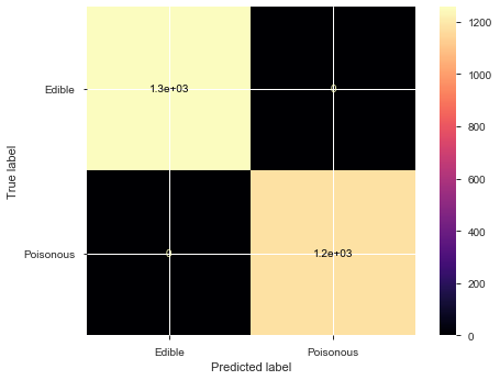
    # To plot confusion matrix
    plot_confusion_matrix(model, X_test, y_test, display_labels=['Edible','Poisonous'], cmap='magma')
    plt.show(block=False)
    
    # To display classification report showing precision, recall, f1
    print('-'*80)
    print('Classification report :\n')
    print(classification_report(y_test, y_predict))
    print('-'*80)

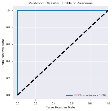
    # To plot roc_auc graph to show area under the curve
    print('ROC_AUC score :')
    print(round(roc_auc_score(y_test, y_prob_predict[:,1]),4))


    fpr, tpr, _ = roc_curve(y_test, y_prob_predict[:,1])
    roc_auc = auc(fpr, tpr)

    plt.figure(figsize=[6,6])
    plt.plot(fpr, tpr, label='ROC curve (area = %0.2f)' % roc_auc, linewidth=4)
    plt.plot([0, 1], [0, 1], 'k--', linewidth=4)
    plt.xlim([-0.05, 1.0])
    plt.ylim([-0.05, 1.05])
    plt.xlabel('False Positive Rate', fontsize=12)
    plt.ylabel('True Positive Rate', fontsize=12)
    plt.title('Mushroom Classifier : Edible or Poisonous', fontsize=12)
    plt.legend(loc="lower right")
    plt.show()

    

for i, model in enumerate(models):   
    
    model_building(model, models_name[i], data_train, data_test, label_train, label_test)

For an initial trial, default parameters were used for all 3 models. The model performances were found good even with the default parameters.

3.1 Model Performance for Logistic RegressionCV

--------------------------------------------------------------------------------
Model Parameters :
LogisticRegressionCV(Cs=10, class_weight=None, cv=None, dual=False,
                     fit_intercept=True, intercept_scaling=1.0, l1_ratios=None,
                     max_iter=100, multi_class='auto', n_jobs=None,
                     penalty='l2', random_state=42, refit=True, scoring=None,
                     solver='lbfgs', tol=0.0001, verbose=0)
--------------------------------------------------------------------------------

--------------------------------------------------------------------------------
Classification report :

              precision    recall  f1-score   support

           0       1.00      1.00      1.00      1257
           1       1.00      1.00      1.00      1181

    accuracy                           1.00      2438
   macro avg       1.00      1.00      1.00      2438
weighted avg       1.00      1.00      1.00      2438

--------------------------------------------------------------------------------
ROC_AUC score :
1.0

3.2 Model Performance for Random Forest Classifier

--------------------------------------------------------------------------------
Model Parameters :
RandomForestClassifier(bootstrap=True, ccp_alpha=0.0, class_weight=None,
                       criterion='gini', max_depth=None, max_features='auto',
                       max_leaf_nodes=None, max_samples=None,
                       min_impurity_decrease=0.0, min_impurity_split=None,
                       min_samples_leaf=1, min_samples_split=2,
                       min_weight_fraction_leaf=0.0, n_estimators=100,
                       n_jobs=None, oob_score=False, random_state=42, verbose=0,
                       warm_start=False)
--------------------------------------------------------------------------------

--------------------------------------------------------------------------------
Classification report :

              precision    recall  f1-score   support

           0       1.00      1.00      1.00      1257
           1       1.00      1.00      1.00      1181

    accuracy                           1.00      2438
   macro avg       1.00      1.00      1.00      2438
weighted avg       1.00      1.00      1.00      2438

--------------------------------------------------------------------------------
ROC_AUC score :
1.0

3.3 Model Performance for KNeighbors Classifier

--------------------------------------------------------------------------------
Model Parameters :
KNeighborsClassifier(algorithm='auto', leaf_size=30, metric='minkowski',
                     metric_params=None, n_jobs=None, n_neighbors=5, p=2,
                     weights='uniform')
--------------------------------------------------------------------------------

--------------------------------------------------------------------------------
Classification report :

              precision    recall  f1-score   support

           0       1.00      1.00      1.00      1257
           1       1.00      1.00      1.00      1181

    accuracy                           1.00      2438
   macro avg       1.00      1.00      1.00      2438
weighted avg       1.00      1.00      1.00      2438

--------------------------------------------------------------------------------
ROC_AUC score :
1.0

Part 4 : Analysis of Feature Importance

To check if there was any variable dominating in predicting the mushroom class and how much the dominance level was, analysis was carried out on the trained models.

4.1 Coefficients derived from Logistic RegressionCV Model

For Logistic RegressionCV, features impact on the model can be extracted by checking the coefficient.

trained_model_lr = joblib.load('./pretrained_models/saved_model_logistic_regressionCV.sav')

# extract feature importance from trained model
feat_importance_lr = trained_model_lr.coef_.tolist()
feat_importance_lr = [round(v, 6) for v in feat_importance_lr[0]]

# set up df for better comparison view
df_feat_importance_lr = pd.DataFrame(data_train.columns, columns=['features'])
df_feat_importance_lr['feature_importance'] = feat_importance_lr
df_feat_importance_lr = df_feat_importance_lr.sort_values('feature_importance', ascending=False)
df_feat_importance_lr

	features	feature_importance
99	spore-print-color_r	6.427334
23	odor_c	4.933256
24	odor_f	4.160369
52	stalk-root_b	3.802192
28	odor_p	3.558643
...	...	...
100	spore-print-color_u	-2.710225
35	gill-size_b	-3.353126
25	odor_l	-4.993461
22	odor_a	-5.036676
27	odor_n	-6.073253

116 rows × 2 columns

To get the top 10 important features, concentation was done to merge the top 5 positive coefficient with top 5 negative coefficient.

df_feat_coef_top10_lr = pd.concat([df_feat_importance_lr.head(5), df_feat_importance_lr.tail(5)])
df_feat_coef_top10_lr.sort_values('feature_importance', ascending=False)

	features	feature_importance
99	spore-print-color_r	6.427334
23	odor_c	4.933256
24	odor_f	4.160369
52	stalk-root_b	3.802192
28	odor_p	3.558643
100	spore-print-color_u	-2.710225
35	gill-size_b	-3.353126
25	odor_l	-4.993461
22	odor_a	-5.036676
27	odor_n	-6.073253

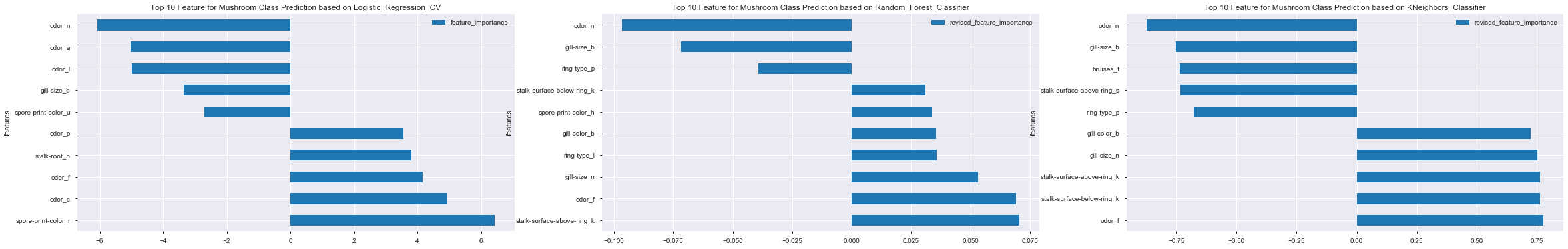
df_feat_coef_top10_lr.plot(x='features', y='feature_importance', kind='barh', figsize=(12,6))
plt.title('Top 10 Feature for Mushroom Class Prediction based on Logistic_Regression_CV')
plt.show()

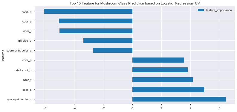
• No particular feature showing dominant effect on mushroom class prediction
• In general, combination of odor, gill-size and spore-print-color demonstrated higher effects on final mushroom class prediction

4.2 Feature Importance derived from Random Forest Classifier Model

Different from Logistic RegressionCV, to identify contributing features, feature importance was extracted out from Random Forest model.

trained_model_rf = joblib.load('./pretrained_models/saved_model_random_forest_classifier.sav')

# extract feature importance from trained model
feat_importance_rf = list(trained_model_rf.feature_importances_)
feat_importance_rf = [round(v, 6) for v in feat_importance_rf]

# set up df for better comparison view
df_feat_importance_rf = pd.DataFrame(data_train.columns, columns=['features'])
df_feat_importance_rf['feature_importance'] = feat_importance_rf
df_feat_importance_rf.sort_values('feature_importance', ascending=False)

	features	feature_importance
27	odor_n	0.096636
35	gill-size_b	0.071668
57	stalk-surface-above-ring_k	0.070451
24	odor_f	0.069137
36	gill-size_n	0.053173
...	...	...
66	stalk-color-above-ring_e	0.000009
98	spore-print-color_o	0.000000
102	spore-print-color_y	0.000000
94	spore-print-color_b	0.000000
43	gill-color_o	0.000000

116 rows × 2 columns

df_feat_imp_top10 = df_feat_importance_rf.sort_values('feature_importance', ascending=False).head(10)
df_feat_imp_top10

	features	feature_importance
27	odor_n	0.096636
35	gill-size_b	0.071668
57	stalk-surface-above-ring_k	0.070451
24	odor_f	0.069137
36	gill-size_n	0.053173
93	ring-type_p	0.039158
91	ring-type_l	0.035865
37	gill-color_b	0.035587
95	spore-print-color_h	0.033872
61	stalk-surface-below-ring_k	0.031121

These values were found standard-scaled to the range of 0 to 1. Even after a selection of the top 10 feature, as there was no sign of +ve or -ve from these feature importance values, we would not be able to gauge if these top 10 feature was positively or negatively affecting the mushroom class prediction. To solve this problem, the correlation table generated earlier in Part 2 was used as a reference.

# re-setup df to reflect which feature importance is positively or negatively affecting the mushroom class prediction
df_feat_imp_correlation_top10_rf = df_feat_imp_top10.merge(df_feature_correlation, how='inner', left_on='features', right_on='features')
df_feat_imp_correlation_top10_rf

	features	feature_importance	correlation_to_class
0	odor_n	0.096636	-0.785557
1	gill-size_b	0.071668	-0.540024
2	stalk-surface-above-ring_k	0.070451	0.587658
3	odor_f	0.069137	0.623842
4	gill-size_n	0.053173	0.540024
5	ring-type_p	0.039158	-0.540469
6	ring-type_l	0.035865	0.451619
7	gill-color_b	0.035587	0.538808
8	spore-print-color_h	0.033872	0.490229
9	stalk-surface-below-ring_k	0.031121	0.573524

By utilizing the +ve / -ve sign from the correlation_to_class column, it was then used as a reference sign to turn the original feature_important values into either a positive or negative value. WIth this method, the original weight of the feature important was retained and it was further enhanced to have an indication sign to show whether these features increased or decreased their importance affecting the class prediction.

df_feat_imp_correlation_top10_rf['revised_feature_importance'] = np.where(df_feat_imp_correlation_top10_rf['correlation_to_class']<0, -1*df_feat_imp_correlation_top10_rf['feature_importance'], df_feat_imp_correlation_top10_rf['feature_importance'])
df_feat_imp_correlation_top10_rf = df_feat_imp_correlation_top10_rf.sort_values(by='revised_feature_importance', ascending=False)
df_feat_imp_correlation_top10_rf

	features	feature_importance	correlation_to_class	revised_feature_importance
2	stalk-surface-above-ring_k	0.070451	0.587658	0.070451
3	odor_f	0.069137	0.623842	0.069137
4	gill-size_n	0.053173	0.540024	0.053173
6	ring-type_l	0.035865	0.451619	0.035865
7	gill-color_b	0.035587	0.538808	0.035587
8	spore-print-color_h	0.033872	0.490229	0.033872
9	stalk-surface-below-ring_k	0.031121	0.573524	0.031121
5	ring-type_p	0.039158	-0.540469	-0.039158
1	gill-size_b	0.071668	-0.540024	-0.071668
0	odor_n	0.096636	-0.785557	-0.096636

df_feat_imp_correlation_top10_rf.plot(x='features', y='revised_feature_importance', kind='barh', figsize=(12,6))
plt.title('Top 10 Feature for Mushroom Class Prediction based on Random_Forest_Classifier')
plt.show()

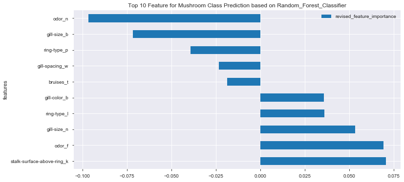
• No particular feature showing dominant effect on mushroom class prediction
• In general, combination of odor, gill-size, ring-type and stalk-surface demonstrated higher effects on final mushroom class prediction

4.3 Feature Importance derived from KNeighbors Classifier

As compared to Logistic RegressionCV and Random Forest Classifier, there’s no coefficient or feature importance that can be extracted easily from the trained model for Kneighbors Classifier. One way to quantitatively check which feature has greater impact is to perform n_features classification using ONE single feature at a time.

trained_model_kn = joblib.load('./pretrained_models/saved_model_kneighbors_classifier.sav')

features = data_test.columns

master_score_list = []

# iterate through each feature to check cross_val_score to find which features having higher score
for i, feature in enumerate(features):
    data_single_feature = np.array(data_test.iloc[:, i]).reshape(-1, 1)
    score_single_feature = cross_val_score(model_kn, data_single_feature, label_test, cv=3)
    mean_score = np.mean(score_single_feature)
    master_score_list.append(mean_score)
    
df_kNeighbors_feature_score = pd.DataFrame()
df_kNeighbors_feature_score['features'] = data_test.columns
df_kNeighbors_feature_score['cross_val_score_single_feature'] = master_score_list
df_kNeighbors_feature_score_top10 = df_kNeighbors_feature_score.sort_values('cross_val_score_single_feature', ascending=False).head(10)
df_kNeighbors_feature_score_top10

	features	cross_val_score_single_feature
27	odor_n	0.876126
24	odor_f	0.779325
61	stalk-surface-below-ring_k	0.763336
57	stalk-surface-above-ring_k	0.763333
36	gill-size_n	0.752266
35	gill-size_b	0.752266
21	bruises_t	0.735438
58	stalk-surface-above-ring_s	0.733388
37	gill-color_b	0.725599
93	ring-type_p	0.677935

Similar as Random Forest Classifier feature importanct study in Part 4.2, the cross validation score doesn’t have a +ve or -ve values. Therefore, the correlation_to_class column was merged in order to utilize its sign to convert the cross-val-score values.

# re-setup df to reflect which feature importance is carrying a postive or negative effect
df_feat_score_correlation_top10_kn = df_kNeighbors_feature_score_top10.merge(df_feature_correlation, how='inner', left_on='features', right_on='features')
df_feat_score_correlation_top10_kn

	features	cross_val_score_single_feature	correlation_to_class
0	odor_n	0.876126	-0.785557
1	odor_f	0.779325	0.623842
2	stalk-surface-below-ring_k	0.763336	0.573524
3	stalk-surface-above-ring_k	0.763333	0.587658
4	gill-size_n	0.752266	0.540024
5	gill-size_b	0.752266	-0.540024
6	bruises_t	0.735438	-0.501530
7	stalk-surface-above-ring_s	0.733388	-0.491314
8	gill-color_b	0.725599	0.538808
9	ring-type_p	0.677935	-0.540469

# utilize the correlation values to generate revised feature importances that reflect either having positive or negative effect

df_feat_score_correlation_top10_kn['revised_feature_importance'] = np.where(df_feat_score_correlation_top10_kn['correlation_to_class']<0, -1*df_feat_score_correlation_top10_kn['cross_val_score_single_feature'], df_feat_score_correlation_top10_kn['cross_val_score_single_feature'])
df_feat_score_correlation_top10_kn = df_feat_score_correlation_top10_kn.sort_values(by='revised_feature_importance', ascending=False)
df_feat_score_correlation_top10_kn

	features	cross_val_score_single_feature	correlation_to_class	revised_feature_importance
1	odor_f	0.779325	0.623842	0.779325
2	stalk-surface-below-ring_k	0.763336	0.573524	0.763336
3	stalk-surface-above-ring_k	0.763333	0.587658	0.763333
4	gill-size_n	0.752266	0.540024	0.752266
8	gill-color_b	0.725599	0.538808	0.725599
9	ring-type_p	0.677935	-0.540469	-0.677935
7	stalk-surface-above-ring_s	0.733388	-0.491314	-0.733388
6	bruises_t	0.735438	-0.501530	-0.735438
5	gill-size_b	0.752266	-0.540024	-0.752266
0	odor_n	0.876126	-0.785557	-0.876126

df_feat_score_correlation_top10_kn.plot(x='features', y='revised_feature_importance', kind='barh', figsize=(12,6))
plt.title('Top 10 Feature for Mushroom Class Prediction based on KNeighbors_Classifier')
plt.show()

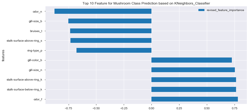
• No particular feature showing dominant effect on mushroom class prediction
• In general, combination of odor, gill-size and stalk-surface demonstrated higher effects on final mushroom class prediction

4.4 Common Top Feature across Difference Models

To find common top features that appear in all 3 models, simply iterate through features and feature-related dataframe

# find common top feature that appears in all 3 models

for feat in list(df_feat_coef_top10_lr['features']):
    if (feat in list(df_feat_imp_correlation_top10_rf['features'])) and \
        (feat in list(df_feat_score_correlation_top10_kn['features'])):
        print(feat)

The print results showed common Top Features for all the evaluated models as follows:

odor_f
gill-size_b
odor_n

Part 5 : Conclusion

From the model preformance, all 3 evaluated models were found having good accuracy and F1 score. However, as these models were computed based on different algorithms, the feature importance extracted / identified from the models were therefore different. Consistency was observed in both odor and gill-size features in term of their influencing patterns :

• odor_f (foul) => positively influece the class prediction [ high tendency output as ‘poisonous’ ]
• gill-size_b (broad) and odor_n (none) => negatively influence the class prediction [ high tendency output as ‘edible’ ]

For highest safety and precautionary steps, it is still advisable to compare the mushroom class prediction for all 3 models. Only if all 3 models showing the same output predictions, the edibility of the mushroom is then best classified.

Extras : Deployment

For fast check on the models and its class prediction, you may check the link HERE