![]()
This is another exercise to practise EDA using various techniques. Dataset was obtained from Public Source. The challenge for this dataset is its size. It only has 17 rows but with 28 columns. Different thought process is required in order to process this type of data.
Package imports
import numpy as np
import scipy.stats as stats
import statsmodels.api as sm
import csv
import pandas as pd
import seaborn as sns
import matplotlib.pyplot as plt

plt.rcParams["patch.force_edgecolor"] = True
sns.set(style='darkgrid')
%matplotlib inline
%config InlineBackend.figure_format = 'retina'
Part 1 : Data Loading and Cleaning
To check if there are any anomalies on the dataset, and if transformation is needed
pd.set_option('max_columns',50)
drug = pd.read_csv('./drug-use-by-age.csv')
print(drug.shape)
drug.head()
(17, 28)
| age | n | alcohol-use | alcohol-frequency | marijuana-use | marijuana-frequency | cocaine-use | cocaine-frequency | crack-use | crack-frequency | heroin-use | heroin-frequency | hallucinogen-use | hallucinogen-frequency | inhalant-use | inhalant-frequency | pain-releiver-use | pain-releiver-frequency | oxycontin-use | oxycontin-frequency | tranquilizer-use | tranquilizer-frequency | stimulant-use | stimulant-frequency | meth-use | meth-frequency | sedative-use | sedative-frequency | |
|---|---|---|---|---|---|---|---|---|---|---|---|---|---|---|---|---|---|---|---|---|---|---|---|---|---|---|---|---|
| 0 | 12 | 2798 | 3.9 | 3.0 | 1.1 | 4.0 | 0.1 | 5.0 | 0.0 | - | 0.1 | 35.5 | 0.2 | 52.0 | 1.6 | 19.0 | 2.0 | 36.0 | 0.1 | 24.5 | 0.2 | 52.0 | 0.2 | 2.0 | 0.0 | - | 0.2 | 13.0 |
| 1 | 13 | 2757 | 8.5 | 6.0 | 3.4 | 15.0 | 0.1 | 1.0 | 0.0 | 3.0 | 0.0 | - | 0.6 | 6.0 | 2.5 | 12.0 | 2.4 | 14.0 | 0.1 | 41.0 | 0.3 | 25.5 | 0.3 | 4.0 | 0.1 | 5.0 | 0.1 | 19.0 |
| 2 | 14 | 2792 | 18.1 | 5.0 | 8.7 | 24.0 | 0.1 | 5.5 | 0.0 | - | 0.1 | 2.0 | 1.6 | 3.0 | 2.6 | 5.0 | 3.9 | 12.0 | 0.4 | 4.5 | 0.9 | 5.0 | 0.8 | 12.0 | 0.1 | 24.0 | 0.2 | 16.5 |
| 3 | 15 | 2956 | 29.2 | 6.0 | 14.5 | 25.0 | 0.5 | 4.0 | 0.1 | 9.5 | 0.2 | 1.0 | 2.1 | 4.0 | 2.5 | 5.5 | 5.5 | 10.0 | 0.8 | 3.0 | 2.0 | 4.5 | 1.5 | 6.0 | 0.3 | 10.5 | 0.4 | 30.0 |
| 4 | 16 | 3058 | 40.1 | 10.0 | 22.5 | 30.0 | 1.0 | 7.0 | 0.0 | 1.0 | 0.1 | 66.5 | 3.4 | 3.0 | 3.0 | 3.0 | 6.2 | 7.0 | 1.1 | 4.0 | 2.4 | 11.0 | 1.8 | 9.5 | 0.3 | 36.0 | 0.2 | 3.0 |
- This is a ‘short & fat’ dataset consists of only 17 rows but with 28 columns.
- cleaning is required
- missing values are observed for some columns
drug.info()
<class 'pandas.core.frame.DataFrame'>
RangeIndex: 17 entries, 0 to 16
Data columns (total 28 columns):
age                        17 non-null object
n                          17 non-null int64
alcohol-use                17 non-null float64
alcohol-frequency          17 non-null float64
marijuana-use              17 non-null float64
marijuana-frequency        17 non-null float64
cocaine-use                17 non-null float64
cocaine-frequency          17 non-null object
crack-use                  17 non-null float64
crack-frequency            17 non-null object
heroin-use                 17 non-null float64
heroin-frequency           17 non-null object
hallucinogen-use           17 non-null float64
hallucinogen-frequency     17 non-null float64
inhalant-use               17 non-null float64
inhalant-frequency         17 non-null object
pain-releiver-use          17 non-null float64
pain-releiver-frequency    17 non-null float64
oxycontin-use              17 non-null float64
oxycontin-frequency        17 non-null object
tranquilizer-use           17 non-null float64
tranquilizer-frequency     17 non-null float64
stimulant-use              17 non-null float64
stimulant-frequency        17 non-null float64
meth-use                   17 non-null float64
meth-frequency             17 non-null object
sedative-use               17 non-null float64
sedative-frequency         17 non-null float64
dtypes: float64(20), int64(1), object(7)
memory usage: 3.8+ KB
- some numerical values are in wrong data types (object -> float)
Columns with data type=object are examined further in order to understand why it is turned to object data type whilst it actually contains numeric values
print('Age : {}'.format(drug['age'].unique()))
Age : ['12' '13' '14' '15' '16' '17' '18' '19' '20' '21' '22-23' '24-25' '26-29'
 '30-34' '35-49' '50-64' '65+']
- some values in Age column are in discrete values whilst some in range (but inconsistent range interval), one is found having special character (+)
print('cocaine-frequency : {}'.format(drug['cocaine-frequency'].unique()))
print('crack-frequency : {}'.format(drug['crack-frequency'].unique()))
print('heroin-frequency : {}'.format(drug['heroin-frequency'].unique()))
print('inhalant-frequency : {}'.format(drug['inhalant-frequency'].unique()))
print('oxycontin-frequency : {}'.format(drug['oxycontin-frequency'].unique()))
print('meth-frequency: {}'.format(drug['meth-frequency'].unique()))
cocaine-frequency : ['5.0' '1.0' '5.5' '4.0' '7.0' '8.0' '6.0' '15.0' '36.0' '-']
crack-frequency : ['-' '3.0' '9.5' '1.0' '21.0' '10.0' '2.0' '5.0' '17.0' '6.0' '15.0'
 '48.0' '62.0']
heroin-frequency : ['35.5' '-' '2.0' '1.0' '66.5' '64.0' '46.0' '180.0' '45.0' '30.0' '57.5'
 '88.0' '50.0' '66.0' '280.0' '41.0' '120.0']
inhalant-frequency : ['19.0' '12.0' '5.0' '5.5' '3.0' '4.0' '2.0' '3.5' '10.0' '13.5' '-']
oxycontin-frequency : ['24.5' '41.0' '4.5' '3.0' '4.0' '6.0' '7.0' '7.5' '12.0' '13.5' '17.5'
 '20.0' '46.0' '5.0' '-']
meth-frequency: ['-' '5.0' '24.0' '10.5' '36.0' '48.0' '12.0' '105.0' '2.0' '46.0' '21.0'
 '30.0' '54.0' '104.0']
- some missing values are observed with ‘-‘
Extraction of records with ‘-‘
drug[drug.values =='-']
| age | n | alcohol-use | alcohol-frequency | marijuana-use | marijuana-frequency | cocaine-use | cocaine-frequency | crack-use | crack-frequency | heroin-use | heroin-frequency | hallucinogen-use | hallucinogen-frequency | inhalant-use | inhalant-frequency | pain-releiver-use | pain-releiver-frequency | oxycontin-use | oxycontin-frequency | tranquilizer-use | tranquilizer-frequency | stimulant-use | stimulant-frequency | meth-use | meth-frequency | sedative-use | sedative-frequency | |
|---|---|---|---|---|---|---|---|---|---|---|---|---|---|---|---|---|---|---|---|---|---|---|---|---|---|---|---|---|
| 0 | 12 | 2798 | 3.9 | 3.0 | 1.1 | 4.0 | 0.1 | 5.0 | 0.0 | - | 0.1 | 35.5 | 0.2 | 52.0 | 1.6 | 19.0 | 2.0 | 36.0 | 0.1 | 24.5 | 0.2 | 52.0 | 0.2 | 2.0 | 0.0 | - | 0.2 | 13.0 |
| 0 | 12 | 2798 | 3.9 | 3.0 | 1.1 | 4.0 | 0.1 | 5.0 | 0.0 | - | 0.1 | 35.5 | 0.2 | 52.0 | 1.6 | 19.0 | 2.0 | 36.0 | 0.1 | 24.5 | 0.2 | 52.0 | 0.2 | 2.0 | 0.0 | - | 0.2 | 13.0 |
| 1 | 13 | 2757 | 8.5 | 6.0 | 3.4 | 15.0 | 0.1 | 1.0 | 0.0 | 3.0 | 0.0 | - | 0.6 | 6.0 | 2.5 | 12.0 | 2.4 | 14.0 | 0.1 | 41.0 | 0.3 | 25.5 | 0.3 | 4.0 | 0.1 | 5.0 | 0.1 | 19.0 |
| 2 | 14 | 2792 | 18.1 | 5.0 | 8.7 | 24.0 | 0.1 | 5.5 | 0.0 | - | 0.1 | 2.0 | 1.6 | 3.0 | 2.6 | 5.0 | 3.9 | 12.0 | 0.4 | 4.5 | 0.9 | 5.0 | 0.8 | 12.0 | 0.1 | 24.0 | 0.2 | 16.5 |
| 16 | 65+ | 2448 | 49.3 | 52.0 | 1.2 | 36.0 | 0.0 | - | 0.0 | - | 0.0 | 120.0 | 0.1 | 2.0 | 0.0 | - | 0.6 | 24.0 | 0.0 | - | 0.2 | 5.0 | 0.0 | 364.0 | 0.0 | - | 0.0 | 15.0 |
| 16 | 65+ | 2448 | 49.3 | 52.0 | 1.2 | 36.0 | 0.0 | - | 0.0 | - | 0.0 | 120.0 | 0.1 | 2.0 | 0.0 | - | 0.6 | 24.0 | 0.0 | - | 0.2 | 5.0 | 0.0 | 364.0 | 0.0 | - | 0.0 | 15.0 |
| 16 | 65+ | 2448 | 49.3 | 52.0 | 1.2 | 36.0 | 0.0 | - | 0.0 | - | 0.0 | 120.0 | 0.1 | 2.0 | 0.0 | - | 0.6 | 24.0 | 0.0 | - | 0.2 | 5.0 | 0.0 | 364.0 | 0.0 | - | 0.0 | 15.0 |
| 16 | 65+ | 2448 | 49.3 | 52.0 | 1.2 | 36.0 | 0.0 | - | 0.0 | - | 0.0 | 120.0 | 0.1 | 2.0 | 0.0 | - | 0.6 | 24.0 | 0.0 | - | 0.2 | 5.0 | 0.0 | 364.0 | 0.0 | - | 0.0 | 15.0 |
| 16 | 65+ | 2448 | 49.3 | 52.0 | 1.2 | 36.0 | 0.0 | - | 0.0 | - | 0.0 | 120.0 | 0.1 | 2.0 | 0.0 | - | 0.6 | 24.0 | 0.0 | - | 0.2 | 5.0 | 0.0 | 364.0 | 0.0 | - | 0.0 | 15.0 |
Replacement of cells with ‘-‘ to NA values
drug.replace('-', np.nan, inplace=True)
drug.head()
| age | n | alcohol-use | alcohol-frequency | marijuana-use | marijuana-frequency | cocaine-use | cocaine-frequency | crack-use | crack-frequency | heroin-use | heroin-frequency | hallucinogen-use | hallucinogen-frequency | inhalant-use | inhalant-frequency | pain-releiver-use | pain-releiver-frequency | oxycontin-use | oxycontin-frequency | tranquilizer-use | tranquilizer-frequency | stimulant-use | stimulant-frequency | meth-use | meth-frequency | sedative-use | sedative-frequency | |
|---|---|---|---|---|---|---|---|---|---|---|---|---|---|---|---|---|---|---|---|---|---|---|---|---|---|---|---|---|
| 0 | 12 | 2798 | 3.9 | 3.0 | 1.1 | 4.0 | 0.1 | 5.0 | 0.0 | NaN | 0.1 | 35.5 | 0.2 | 52.0 | 1.6 | 19.0 | 2.0 | 36.0 | 0.1 | 24.5 | 0.2 | 52.0 | 0.2 | 2.0 | 0.0 | NaN | 0.2 | 13.0 |
| 1 | 13 | 2757 | 8.5 | 6.0 | 3.4 | 15.0 | 0.1 | 1.0 | 0.0 | 3.0 | 0.0 | NaN | 0.6 | 6.0 | 2.5 | 12.0 | 2.4 | 14.0 | 0.1 | 41.0 | 0.3 | 25.5 | 0.3 | 4.0 | 0.1 | 5.0 | 0.1 | 19.0 |
| 2 | 14 | 2792 | 18.1 | 5.0 | 8.7 | 24.0 | 0.1 | 5.5 | 0.0 | NaN | 0.1 | 2.0 | 1.6 | 3.0 | 2.6 | 5.0 | 3.9 | 12.0 | 0.4 | 4.5 | 0.9 | 5.0 | 0.8 | 12.0 | 0.1 | 24.0 | 0.2 | 16.5 |
| 3 | 15 | 2956 | 29.2 | 6.0 | 14.5 | 25.0 | 0.5 | 4.0 | 0.1 | 9.5 | 0.2 | 1.0 | 2.1 | 4.0 | 2.5 | 5.5 | 5.5 | 10.0 | 0.8 | 3.0 | 2.0 | 4.5 | 1.5 | 6.0 | 0.3 | 10.5 | 0.4 | 30.0 |
| 4 | 16 | 3058 | 40.1 | 10.0 | 22.5 | 30.0 | 1.0 | 7.0 | 0.0 | 1.0 | 0.1 | 66.5 | 3.4 | 3.0 | 3.0 | 3.0 | 6.2 | 7.0 | 1.1 | 4.0 | 2.4 | 11.0 | 1.8 | 9.5 | 0.3 | 36.0 | 0.2 | 3.0 |
Examination of missing values and data type for each column
drug.isnull().sum()
age                        0
n                          0
alcohol-use                0
alcohol-frequency          0
marijuana-use              0
marijuana-frequency        0
cocaine-use                0
cocaine-frequency          1
crack-use                  0
crack-frequency            3
heroin-use                 0
heroin-frequency           1
hallucinogen-use           0
hallucinogen-frequency     0
inhalant-use               0
inhalant-frequency         1
pain-releiver-use          0
pain-releiver-frequency    0
oxycontin-use              0
oxycontin-frequency        1
tranquilizer-use           0
tranquilizer-frequency     0
stimulant-use              0
stimulant-frequency        0
meth-use                   0
meth-frequency             2
sedative-use               0
sedative-frequency         0
dtype: int64
drug.info()
<class 'pandas.core.frame.DataFrame'>
RangeIndex: 17 entries, 0 to 16
Data columns (total 28 columns):
age                        17 non-null object
n                          17 non-null int64
alcohol-use                17 non-null float64
alcohol-frequency          17 non-null float64
marijuana-use              17 non-null float64
marijuana-frequency        17 non-null float64
cocaine-use                17 non-null float64
cocaine-frequency          16 non-null object
crack-use                  17 non-null float64
crack-frequency            14 non-null object
heroin-use                 17 non-null float64
heroin-frequency           16 non-null object
hallucinogen-use           17 non-null float64
hallucinogen-frequency     17 non-null float64
inhalant-use               17 non-null float64
inhalant-frequency         16 non-null object
pain-releiver-use          17 non-null float64
pain-releiver-frequency    17 non-null float64
oxycontin-use              17 non-null float64
oxycontin-frequency        16 non-null object
tranquilizer-use           17 non-null float64
tranquilizer-frequency     17 non-null float64
stimulant-use              17 non-null float64
stimulant-frequency        17 non-null float64
meth-use                   17 non-null float64
meth-frequency             15 non-null object
sedative-use               17 non-null float64
sedative-frequency         17 non-null float64
dtypes: float64(20), int64(1), object(7)
memory usage: 3.8+ KB
Adjustment of data type to numeric
drug.iloc[:,2:] = drug.iloc[:,2:].astype(float)
drug.dtypes
age                         object
n                            int64
alcohol-use                float64
alcohol-frequency          float64
marijuana-use              float64
marijuana-frequency        float64
cocaine-use                float64
cocaine-frequency          float64
crack-use                  float64
crack-frequency            float64
heroin-use                 float64
heroin-frequency           float64
hallucinogen-use           float64
hallucinogen-frequency     float64
inhalant-use               float64
inhalant-frequency         float64
pain-releiver-use          float64
pain-releiver-frequency    float64
oxycontin-use              float64
oxycontin-frequency        float64
tranquilizer-use           float64
tranquilizer-frequency     float64
stimulant-use              float64
stimulant-frequency        float64
meth-use                   float64
meth-frequency             float64
sedative-use               float64
sedative-frequency         float64
dtype: object
drug.describe()
| n | alcohol-use | alcohol-frequency | marijuana-use | marijuana-frequency | cocaine-use | cocaine-frequency | crack-use | crack-frequency | heroin-use | heroin-frequency | hallucinogen-use | hallucinogen-frequency | inhalant-use | inhalant-frequency | pain-releiver-use | pain-releiver-frequency | oxycontin-use | oxycontin-frequency | tranquilizer-use | tranquilizer-frequency | stimulant-use | stimulant-frequency | meth-use | meth-frequency | sedative-use | sedative-frequency | |
|---|---|---|---|---|---|---|---|---|---|---|---|---|---|---|---|---|---|---|---|---|---|---|---|---|---|---|---|
| count | 17.000000 | 17.000000 | 17.000000 | 17.000000 | 17.000000 | 17.000000 | 16.000000 | 17.000000 | 14.000000 | 17.000000 | 16.000000 | 17.000000 | 17.000000 | 17.000000 | 16.000000 | 17.000000 | 17.000000 | 17.000000 | 16.000000 | 17.000000 | 17.000000 | 17.000000 | 17.000000 | 17.000000 | 15.000000 | 17.000000 | 17.000000 |
| mean | 3251.058824 | 55.429412 | 33.352941 | 18.923529 | 42.941176 | 2.176471 | 7.875000 | 0.294118 | 15.035714 | 0.352941 | 73.281250 | 3.394118 | 8.411765 | 1.388235 | 6.156250 | 6.270588 | 14.705882 | 0.935294 | 14.812500 | 2.805882 | 11.735294 | 1.917647 | 31.147059 | 0.382353 | 35.966667 | 0.282353 | 19.382353 |
| std | 1297.890426 | 26.878866 | 21.318833 | 11.959752 | 18.362566 | 1.816772 | 8.038449 | 0.235772 | 18.111263 | 0.333762 | 70.090173 | 2.792506 | 15.000245 | 0.927283 | 4.860448 | 3.166379 | 6.935098 | 0.608216 | 12.798275 | 1.753379 | 11.485205 | 1.407673 | 85.973790 | 0.262762 | 31.974581 | 0.138000 | 24.833527 |
| min | 2223.000000 | 3.900000 | 3.000000 | 1.100000 | 4.000000 | 0.000000 | 1.000000 | 0.000000 | 1.000000 | 0.000000 | 1.000000 | 0.100000 | 2.000000 | 0.000000 | 2.000000 | 0.600000 | 7.000000 | 0.000000 | 3.000000 | 0.200000 | 4.500000 | 0.000000 | 2.000000 | 0.000000 | 2.000000 | 0.000000 | 3.000000 |
| 25% | 2469.000000 | 40.100000 | 10.000000 | 8.700000 | 30.000000 | 0.500000 | 5.000000 | 0.000000 | 5.000000 | 0.100000 | 39.625000 | 0.600000 | 3.000000 | 0.600000 | 3.375000 | 3.900000 | 12.000000 | 0.400000 | 5.750000 | 1.400000 | 6.000000 | 0.600000 | 7.000000 | 0.200000 | 12.000000 | 0.200000 | 6.500000 |
| 50% | 2798.000000 | 64.600000 | 48.000000 | 20.800000 | 52.000000 | 2.000000 | 5.250000 | 0.400000 | 7.750000 | 0.200000 | 53.750000 | 3.200000 | 3.000000 | 1.400000 | 4.000000 | 6.200000 | 12.000000 | 1.100000 | 12.000000 | 3.500000 | 10.000000 | 1.800000 | 10.000000 | 0.400000 | 30.000000 | 0.300000 | 10.000000 |
| 75% | 3058.000000 | 77.500000 | 52.000000 | 28.400000 | 52.000000 | 4.000000 | 7.250000 | 0.500000 | 16.500000 | 0.600000 | 71.875000 | 5.200000 | 4.000000 | 2.000000 | 6.625000 | 9.000000 | 15.000000 | 1.400000 | 18.125000 | 4.200000 | 11.000000 | 3.000000 | 12.000000 | 0.600000 | 47.000000 | 0.400000 | 17.500000 |
| max | 7391.000000 | 84.200000 | 52.000000 | 34.000000 | 72.000000 | 4.900000 | 36.000000 | 0.600000 | 62.000000 | 1.100000 | 280.000000 | 8.600000 | 52.000000 | 3.000000 | 19.000000 | 10.000000 | 36.000000 | 1.700000 | 46.000000 | 5.400000 | 52.000000 | 4.100000 | 364.000000 | 0.900000 | 105.000000 | 0.500000 | 104.000000 |
- some columns show high standard deviation values
Part 2 : High Level Overview of Data
2.1 : Check age group vs sample size distribution
drug.plot.bar(x='age', y='n', figsize=(15,6), color='grey')
plt.title('Distribution of Sample Size by Age')
plt.ylabel('sample size')
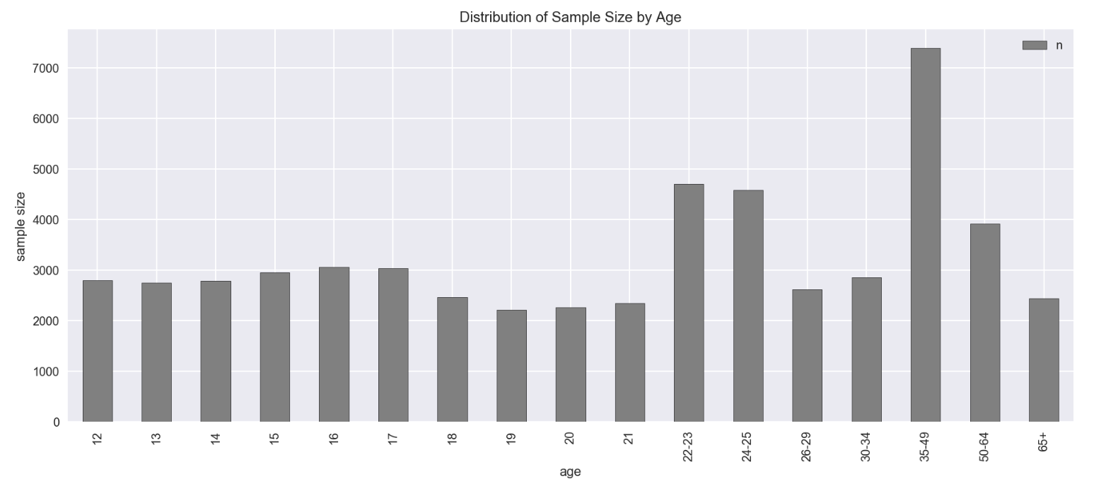
- Sample size for age from 12-21 is more stable ranging from 2000 to 3000+
- for age from 12 - 17 is around +/-3000
- for age from 18 - 21 is around +/-2500
- Sample size for other age groups varies a lot. Data showed inconsistency in age group from 22 onwards
2.2 : For better comparison and avoid misleading graph interpretation due to mixture of age vs age groups, convert age group into average
def age_modified(age):
    if '+' in age:
        age = float(age.strip('+'))
    elif '-' in age:
        x = age.split('-')
        age = (float(x[1]) - float(x[0]))/2. + float(x[0])
    else:
        age = float(age)
    return age
drug['age'] = drug['age'].apply(age_modified)
drug
| age | n | alcohol-use | alcohol-frequency | marijuana-use | marijuana-frequency | cocaine-use | cocaine-frequency | crack-use | crack-frequency | heroin-use | heroin-frequency | hallucinogen-use | hallucinogen-frequency | inhalant-use | inhalant-frequency | pain-releiver-use | pain-releiver-frequency | oxycontin-use | oxycontin-frequency | tranquilizer-use | tranquilizer-frequency | stimulant-use | stimulant-frequency | meth-use | meth-frequency | sedative-use | sedative-frequency | |
|---|---|---|---|---|---|---|---|---|---|---|---|---|---|---|---|---|---|---|---|---|---|---|---|---|---|---|---|---|
| 0 | 12.0 | 2798 | 3.9 | 3.0 | 1.1 | 4.0 | 0.1 | 5.0 | 0.0 | NaN | 0.1 | 35.5 | 0.2 | 52.0 | 1.6 | 19.0 | 2.0 | 36.0 | 0.1 | 24.5 | 0.2 | 52.0 | 0.2 | 2.0 | 0.0 | NaN | 0.2 | 13.0 |
| 1 | 13.0 | 2757 | 8.5 | 6.0 | 3.4 | 15.0 | 0.1 | 1.0 | 0.0 | 3.0 | 0.0 | NaN | 0.6 | 6.0 | 2.5 | 12.0 | 2.4 | 14.0 | 0.1 | 41.0 | 0.3 | 25.5 | 0.3 | 4.0 | 0.1 | 5.0 | 0.1 | 19.0 |
| 2 | 14.0 | 2792 | 18.1 | 5.0 | 8.7 | 24.0 | 0.1 | 5.5 | 0.0 | NaN | 0.1 | 2.0 | 1.6 | 3.0 | 2.6 | 5.0 | 3.9 | 12.0 | 0.4 | 4.5 | 0.9 | 5.0 | 0.8 | 12.0 | 0.1 | 24.0 | 0.2 | 16.5 |
| 3 | 15.0 | 2956 | 29.2 | 6.0 | 14.5 | 25.0 | 0.5 | 4.0 | 0.1 | 9.5 | 0.2 | 1.0 | 2.1 | 4.0 | 2.5 | 5.5 | 5.5 | 10.0 | 0.8 | 3.0 | 2.0 | 4.5 | 1.5 | 6.0 | 0.3 | 10.5 | 0.4 | 30.0 |
| 4 | 16.0 | 3058 | 40.1 | 10.0 | 22.5 | 30.0 | 1.0 | 7.0 | 0.0 | 1.0 | 0.1 | 66.5 | 3.4 | 3.0 | 3.0 | 3.0 | 6.2 | 7.0 | 1.1 | 4.0 | 2.4 | 11.0 | 1.8 | 9.5 | 0.3 | 36.0 | 0.2 | 3.0 |
| 5 | 17.0 | 3038 | 49.3 | 13.0 | 28.0 | 36.0 | 2.0 | 5.0 | 0.1 | 21.0 | 0.1 | 64.0 | 4.8 | 3.0 | 2.0 | 4.0 | 8.5 | 9.0 | 1.4 | 6.0 | 3.5 | 7.0 | 2.8 | 9.0 | 0.6 | 48.0 | 0.5 | 6.5 |
| 6 | 18.0 | 2469 | 58.7 | 24.0 | 33.7 | 52.0 | 3.2 | 5.0 | 0.4 | 10.0 | 0.4 | 46.0 | 7.0 | 4.0 | 1.8 | 4.0 | 9.2 | 12.0 | 1.7 | 7.0 | 4.9 | 12.0 | 3.0 | 8.0 | 0.5 | 12.0 | 0.4 | 10.0 |
| 7 | 19.0 | 2223 | 64.6 | 36.0 | 33.4 | 60.0 | 4.1 | 5.5 | 0.5 | 2.0 | 0.5 | 180.0 | 8.6 | 3.0 | 1.4 | 3.0 | 9.4 | 12.0 | 1.5 | 7.5 | 4.2 | 4.5 | 3.3 | 6.0 | 0.4 | 105.0 | 0.3 | 6.0 |
| 8 | 20.0 | 2271 | 69.7 | 48.0 | 34.0 | 60.0 | 4.9 | 8.0 | 0.6 | 5.0 | 0.9 | 45.0 | 7.4 | 2.0 | 1.5 | 4.0 | 10.0 | 10.0 | 1.7 | 12.0 | 5.4 | 10.0 | 4.0 | 12.0 | 0.9 | 12.0 | 0.5 | 4.0 |
| 9 | 21.0 | 2354 | 83.2 | 52.0 | 33.0 | 52.0 | 4.8 | 5.0 | 0.5 | 17.0 | 0.6 | 30.0 | 6.3 | 4.0 | 1.4 | 2.0 | 9.0 | 15.0 | 1.3 | 13.5 | 3.9 | 7.0 | 4.1 | 10.0 | 0.6 | 2.0 | 0.3 | 9.0 |
| 10 | 22.5 | 4707 | 84.2 | 52.0 | 28.4 | 52.0 | 4.5 | 5.0 | 0.5 | 5.0 | 1.1 | 57.5 | 5.2 | 3.0 | 1.0 | 4.0 | 10.0 | 15.0 | 1.7 | 17.5 | 4.4 | 12.0 | 3.6 | 10.0 | 0.6 | 46.0 | 0.2 | 52.0 |
| 11 | 24.5 | 4591 | 83.1 | 52.0 | 24.9 | 60.0 | 4.0 | 6.0 | 0.5 | 6.0 | 0.7 | 88.0 | 4.5 | 2.0 | 0.8 | 2.0 | 9.0 | 15.0 | 1.3 | 20.0 | 4.3 | 10.0 | 2.6 | 10.0 | 0.7 | 21.0 | 0.2 | 17.5 |
| 12 | 27.5 | 2628 | 80.7 | 52.0 | 20.8 | 52.0 | 3.2 | 5.0 | 0.4 | 6.0 | 0.6 | 50.0 | 3.2 | 3.0 | 0.6 | 4.0 | 8.3 | 13.0 | 1.2 | 13.5 | 4.2 | 10.0 | 2.3 | 7.0 | 0.6 | 30.0 | 0.4 | 4.0 |
| 13 | 32.0 | 2864 | 77.5 | 52.0 | 16.4 | 72.0 | 2.1 | 8.0 | 0.5 | 15.0 | 0.4 | 66.0 | 1.8 | 2.0 | 0.4 | 3.5 | 5.9 | 22.0 | 0.9 | 46.0 | 3.6 | 8.0 | 1.4 | 12.0 | 0.4 | 54.0 | 0.4 | 10.0 |
| 14 | 42.0 | 7391 | 75.0 | 52.0 | 10.4 | 48.0 | 1.5 | 15.0 | 0.5 | 48.0 | 0.1 | 280.0 | 0.6 | 3.0 | 0.3 | 10.0 | 4.2 | 12.0 | 0.3 | 12.0 | 1.9 | 6.0 | 0.6 | 24.0 | 0.2 | 104.0 | 0.3 | 10.0 |
| 15 | 57.0 | 3923 | 67.2 | 52.0 | 7.3 | 52.0 | 0.9 | 36.0 | 0.4 | 62.0 | 0.1 | 41.0 | 0.3 | 44.0 | 0.2 | 13.5 | 2.5 | 12.0 | 0.4 | 5.0 | 1.4 | 10.0 | 0.3 | 24.0 | 0.2 | 30.0 | 0.2 | 104.0 |
| 16 | 65.0 | 2448 | 49.3 | 52.0 | 1.2 | 36.0 | 0.0 | NaN | 0.0 | NaN | 0.0 | 120.0 | 0.1 | 2.0 | 0.0 | NaN | 0.6 | 24.0 | 0.0 | NaN | 0.2 | 5.0 | 0.0 | 364.0 | 0.0 | NaN | 0.0 | 15.0 |
2.3 : Set up 2 dataframes –> one by drugUse ; one by drugFrequency
drug.columns
Index(['age', 'n', 'alcohol-use', 'alcohol-frequency', 'marijuana-use',
       'marijuana-frequency', 'cocaine-use', 'cocaine-frequency', 'crack-use',
       'crack-frequency', 'heroin-use', 'heroin-frequency', 'hallucinogen-use',
       'hallucinogen-frequency', 'inhalant-use', 'inhalant-frequency',
       'pain-releiver-use', 'pain-releiver-frequency', 'oxycontin-use',
       'oxycontin-frequency', 'tranquilizer-use', 'tranquilizer-frequency',
       'stimulant-use', 'stimulant-frequency', 'meth-use', 'meth-frequency',
       'sedative-use', 'sedative-frequency'],
      dtype='object')
use_columns = [col for col in drug.columns if 'use' in col]
frequency_columns = [col for col in drug.columns if 'frequency' in col]

df_drugUse = drug[use_columns]
df_drugFrequency = drug[frequency_columns]

# insert age column to the front of the new df
df_drugUse.insert(0, 'age', drug['age'] )
df_drugFrequency.insert(0, 'age', drug['age'])
Check if df by drugUse is correctly set up
df_drugUse.head()
| age | alcohol-use | marijuana-use | cocaine-use | crack-use | heroin-use | hallucinogen-use | inhalant-use | pain-releiver-use | oxycontin-use | tranquilizer-use | stimulant-use | meth-use | sedative-use | |
|---|---|---|---|---|---|---|---|---|---|---|---|---|---|---|
| 0 | 12.0 | 3.9 | 1.1 | 0.1 | 0.0 | 0.1 | 0.2 | 1.6 | 2.0 | 0.1 | 0.2 | 0.2 | 0.0 | 0.2 |
| 1 | 13.0 | 8.5 | 3.4 | 0.1 | 0.0 | 0.0 | 0.6 | 2.5 | 2.4 | 0.1 | 0.3 | 0.3 | 0.1 | 0.1 |
| 2 | 14.0 | 18.1 | 8.7 | 0.1 | 0.0 | 0.1 | 1.6 | 2.6 | 3.9 | 0.4 | 0.9 | 0.8 | 0.1 | 0.2 |
| 3 | 15.0 | 29.2 | 14.5 | 0.5 | 0.1 | 0.2 | 2.1 | 2.5 | 5.5 | 0.8 | 2.0 | 1.5 | 0.3 | 0.4 |
| 4 | 16.0 | 40.1 | 22.5 | 1.0 | 0.0 | 0.1 | 3.4 | 3.0 | 6.2 | 1.1 | 2.4 | 1.8 | 0.3 | 0.2 |
Check if df by drugFrequency is correctly set up
df_drugFrequency.head()
| age | alcohol-frequency | marijuana-frequency | cocaine-frequency | crack-frequency | heroin-frequency | hallucinogen-frequency | inhalant-frequency | pain-releiver-frequency | oxycontin-frequency | tranquilizer-frequency | stimulant-frequency | meth-frequency | sedative-frequency | |
|---|---|---|---|---|---|---|---|---|---|---|---|---|---|---|
| 0 | 12.0 | 3.0 | 4.0 | 5.0 | NaN | 35.5 | 52.0 | 19.0 | 36.0 | 24.5 | 52.0 | 2.0 | NaN | 13.0 |
| 1 | 13.0 | 6.0 | 15.0 | 1.0 | 3.0 | NaN | 6.0 | 12.0 | 14.0 | 41.0 | 25.5 | 4.0 | 5.0 | 19.0 |
| 2 | 14.0 | 5.0 | 24.0 | 5.5 | NaN | 2.0 | 3.0 | 5.0 | 12.0 | 4.5 | 5.0 | 12.0 | 24.0 | 16.5 |
| 3 | 15.0 | 6.0 | 25.0 | 4.0 | 9.5 | 1.0 | 4.0 | 5.5 | 10.0 | 3.0 | 4.5 | 6.0 | 10.5 | 30.0 |
| 4 | 16.0 | 10.0 | 30.0 | 7.0 | 1.0 | 66.5 | 3.0 | 3.0 | 7.0 | 4.0 | 11.0 | 9.5 | 36.0 | 3.0 |
2.4a : Visualize data by drugUse in stacked-bar chart
df_drugUse.plot(x='age', kind='bar',stacked=True, figsize=(20,8), colormap='tab20',rot=1)
plt.ylabel('% of population taking the drug')
plt.title('Distribution of Population by Age for Various Drug Types')
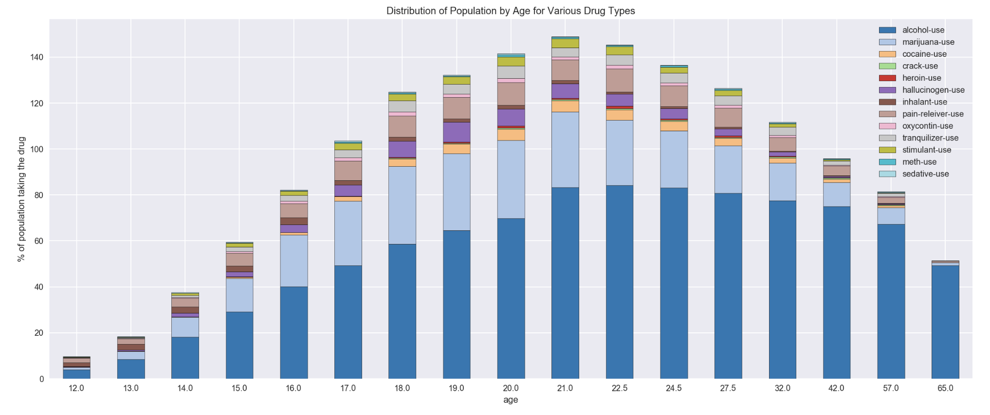
- alcohol is the highest intake in all ages/age groups
- marijuana is the 2nd highest drug intake among various ages/age groups. However, a reduction in marijuana use was observed for age 22 onwards
- pain reliever is the 3rd popular drug with the % of people in the same age/age groups who used this drug remained stable for age 17-21
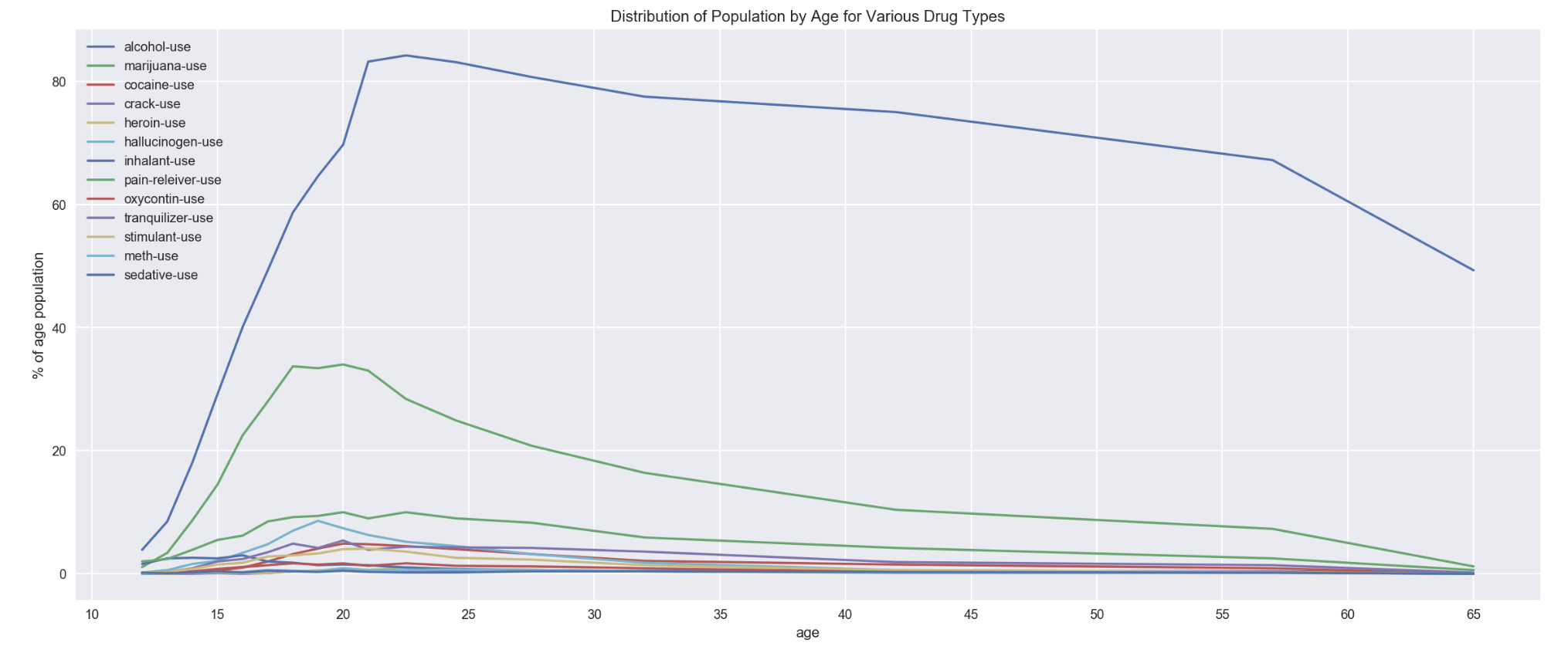
2.4b : Another visualization of drugUse using line chart
df_drugUse.plot('age', xticks=np.arange(10,70,5), figsize=(20,8))
plt.ylabel('% of age population')
plt.title('Distribution of Population by Age for Various Drug Types')
2.5a : Visualization of drug data by Frequency in stacked-bar chart
df_drugFrequency.plot(x='age', figsize=(20,8), stacked=True, kind='bar', colormap='tab20')
plt.ylabel('Frequency')
plt.title('Distribution of Drug Intake Freqeuncy by Age')
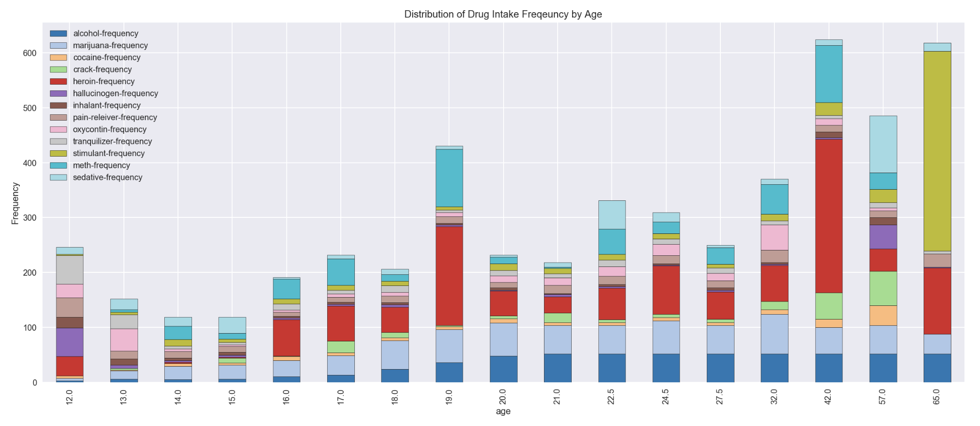
- heroin was the drug with highest frequency of intake age 19 and age group of 35-49
- stimulant was found having a high spike of drug frequency in age group of 65+
- marijuana frequency was found stable for age 18 till age group of 50-64
2.5b : Another visualization of drugFrequency using line chart
df_drugFrequency.plot('age', figsize=(20,8), xticks=np.arange(10,70,5))
plt.ylabel('Median Frequency of Drug Intake')
plt.title('Distribution of Drug Frequency by Age for Various Drug Types')
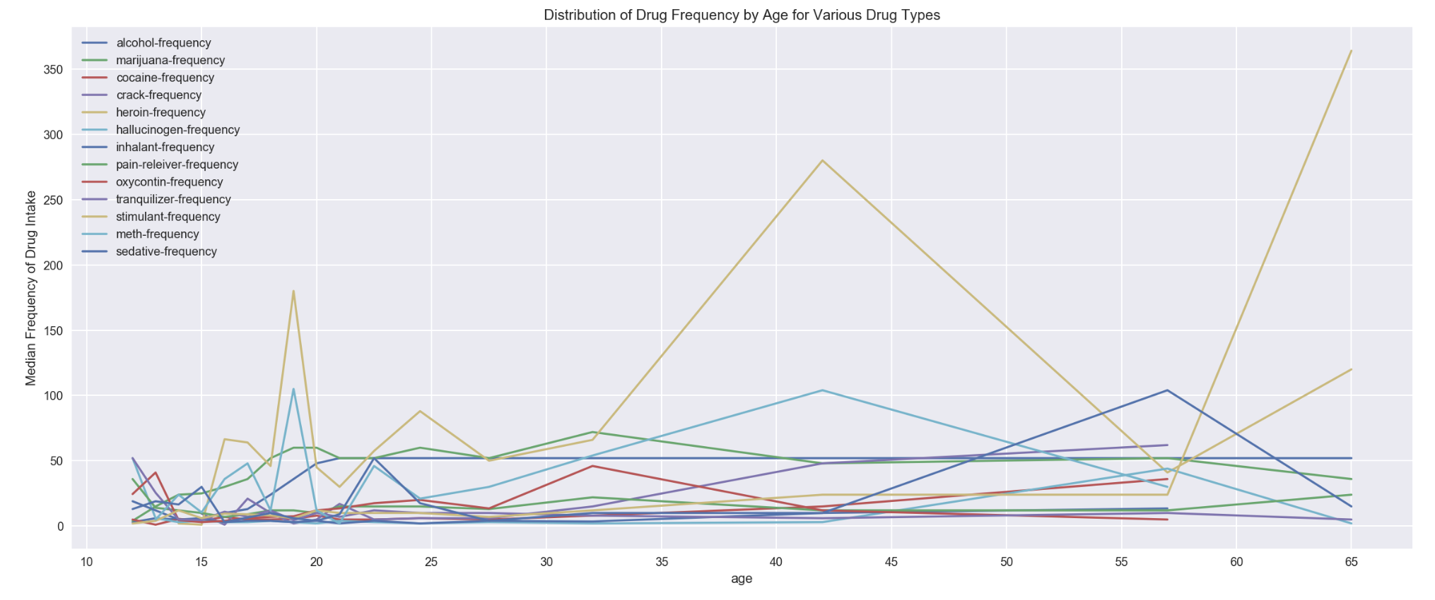
- Visualization through stacked bar gave better comparison view as compared to line plot
2.6 : Check the spread of the data for each category using boxplot
Since data range varies significantly, standardized data before boxplot to enable comparable values on same scale
drugUse_bx = df_drugUse.drop('age', axis=1)
drugFrequency_bx = df_drugFrequency.drop('age', axis=1)

# standardize data on same scale
std_drugUse_bx = (drugUse_bx - drugUse_bx.mean())/drugUse_bx.std()
std_drugFrequency_bx = (drugFrequency_bx - drugFrequency_bx.mean())/drugFrequency_bx.std()
std_drugUse_bx
| alcohol-use | marijuana-use | cocaine-use | crack-use | heroin-use | hallucinogen-use | inhalant-use | pain-releiver-use | oxycontin-use | tranquilizer-use | stimulant-use | meth-use | sedative-use | |
|---|---|---|---|---|---|---|---|---|---|---|---|---|---|
| 0 | -1.917098 | -1.490293 | -1.142945 | -1.247469 | -0.757849 | -1.143818 | 0.228371 | -1.348729 | -1.373352 | -1.486206 | -1.220203 | -1.455128 | -0.596759 |
| 1 | -1.745959 | -1.297981 | -1.142945 | -1.247469 | -1.057464 | -1.000577 | 1.198949 | -1.222402 | -1.373352 | -1.429173 | -1.149164 | -1.074556 | -1.321394 |
| 2 | -1.388802 | -0.854828 | -1.142945 | -1.247469 | -0.757849 | -0.642476 | 1.306791 | -0.748675 | -0.880106 | -1.086977 | -0.793968 | -1.074556 | -0.596759 |
| 3 | -0.975838 | -0.369868 | -0.922774 | -0.823329 | -0.458234 | -0.463425 | 1.198949 | -0.243366 | -0.222444 | -0.459617 | -0.296693 | -0.313412 | 0.852512 |
| 4 | -0.570315 | 0.299042 | -0.647561 | -1.247469 | -0.757849 | 0.002106 | 1.738159 | -0.022293 | 0.270802 | -0.231486 | -0.083576 | -0.313412 | -0.596759 |
| 5 | -0.228038 | 0.758918 | -0.097134 | -0.823329 | -0.757849 | 0.503448 | 0.659739 | 0.704089 | 0.764048 | 0.395874 | 0.626817 | 0.828303 | 1.577148 |
| 6 | 0.121679 | 1.235516 | 0.563378 | 0.449089 | 0.140995 | 1.291271 | 0.444055 | 0.925161 | 1.257294 | 1.194333 | 0.768895 | 0.447732 | 0.852512 |
| 7 | 0.341182 | 1.210432 | 1.058762 | 0.873228 | 0.440610 | 1.864233 | 0.012687 | 0.988325 | 0.928463 | 0.795103 | 0.982013 | 0.067160 | 0.127877 |
| 8 | 0.530922 | 1.260601 | 1.499103 | 1.297367 | 1.639069 | 1.434512 | 0.120529 | 1.177816 | 1.257294 | 1.479496 | 1.479287 | 1.970019 | 1.577148 |
| 9 | 1.033176 | 1.176987 | 1.444061 | 0.873228 | 0.740225 | 1.040600 | 0.012687 | 0.861998 | 0.599632 | 0.624005 | 1.550326 | 0.828303 | 0.127877 |
| 10 | 1.070380 | 0.792363 | 1.278933 | 0.873228 | 2.238298 | 0.646689 | -0.418681 | 1.177816 | 1.257294 | 0.909169 | 1.195130 | 0.828303 | -0.596759 |
| 11 | 1.029455 | 0.499715 | 1.003719 | 0.873228 | 1.039839 | 0.396018 | -0.634365 | 0.861998 | 0.599632 | 0.852136 | 0.484738 | 1.208875 | -0.596759 |
| 12 | 0.940166 | 0.156899 | 0.563378 | 0.449089 | 0.740225 | -0.069514 | -0.850049 | 0.640925 | 0.435217 | 0.795103 | 0.271621 | 0.828303 | 0.852512 |
| 13 | 0.821113 | -0.211002 | -0.042091 | 0.873228 | 0.140995 | -0.570856 | -1.065733 | -0.117038 | -0.058029 | 0.452907 | -0.367732 | 0.067160 | 0.852512 |
| 14 | 0.728103 | -0.712684 | -0.372347 | 0.873228 | -0.757849 | -1.000577 | -1.173575 | -0.653929 | -1.044521 | -0.516649 | -0.936046 | -0.693984 | 0.127877 |
| 15 | 0.437912 | -0.971887 | -0.702603 | 0.449089 | -0.757849 | -1.108008 | -1.281417 | -1.190820 | -0.880106 | -0.801813 | -1.149164 | -0.693984 | -0.596759 |
| 16 | -0.228038 | -1.481931 | -1.197988 | -1.247469 | -1.057464 | -1.179628 | -1.497101 | -1.790875 | -1.537767 | -1.486206 | -1.362281 | -1.455128 | -2.046029 |
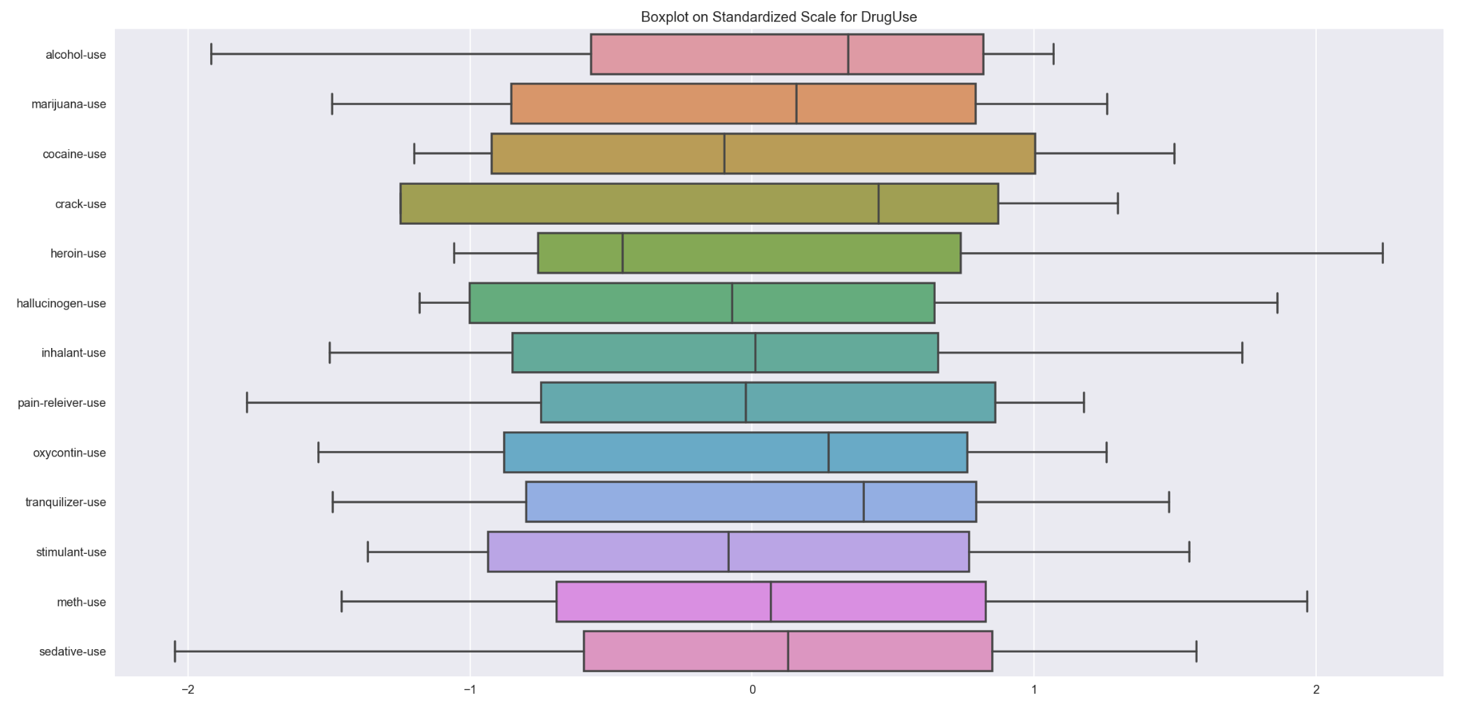
Comparision of various drugUse spread on same scale
plt.figure(figsize=(20,10))
sns.boxplot(data=std_drugUse_bx, orient='h',)
plt.title('Boxplot on Standardized Scale for DrugUse')
Comparision of various drugFrequency spread on same scale
plt.figure(figsize=(20,10))
sns.boxplot(data=std_drugFrequency_bx, orient='h')
plt.title('Boxplot on Standardized Scale for DrugFrequency')
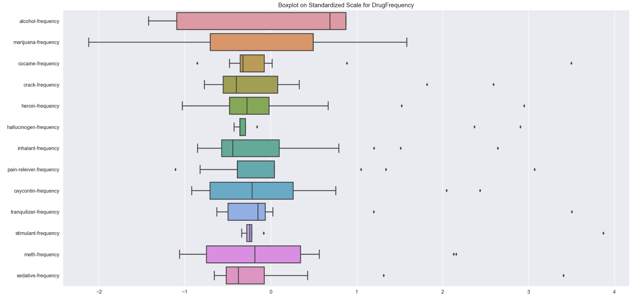
- drugFrequency data is more scatter and with more outliers as compared to drugUse data
2.7a : Check the correlation of data in drugUse dataset
drugUse_temp = df_drugUse.drop('age', axis=1)
drugFrequency_temp = df_drugFrequency.drop('age', axis=1)
plt.figure(figsize=(12,8))
sns.heatmap(drugUse_temp.corr(),cmap='RdBu_r',annot=True)
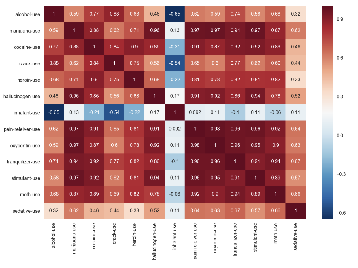
- inhalant-use has almost no to negative correlation to the rest of the drug use
- other drug-use are generally having positive correlation to each other in different levels
Visualization of the correlation of top 4 popular drugs (alcohol, marijuana, hallucinogen, and pain-reliever)
sns.pairplot(drugUse_temp[['alcohol-use','marijuana-use','hallucinogen-use','pain-releiver-use']],kind='reg')
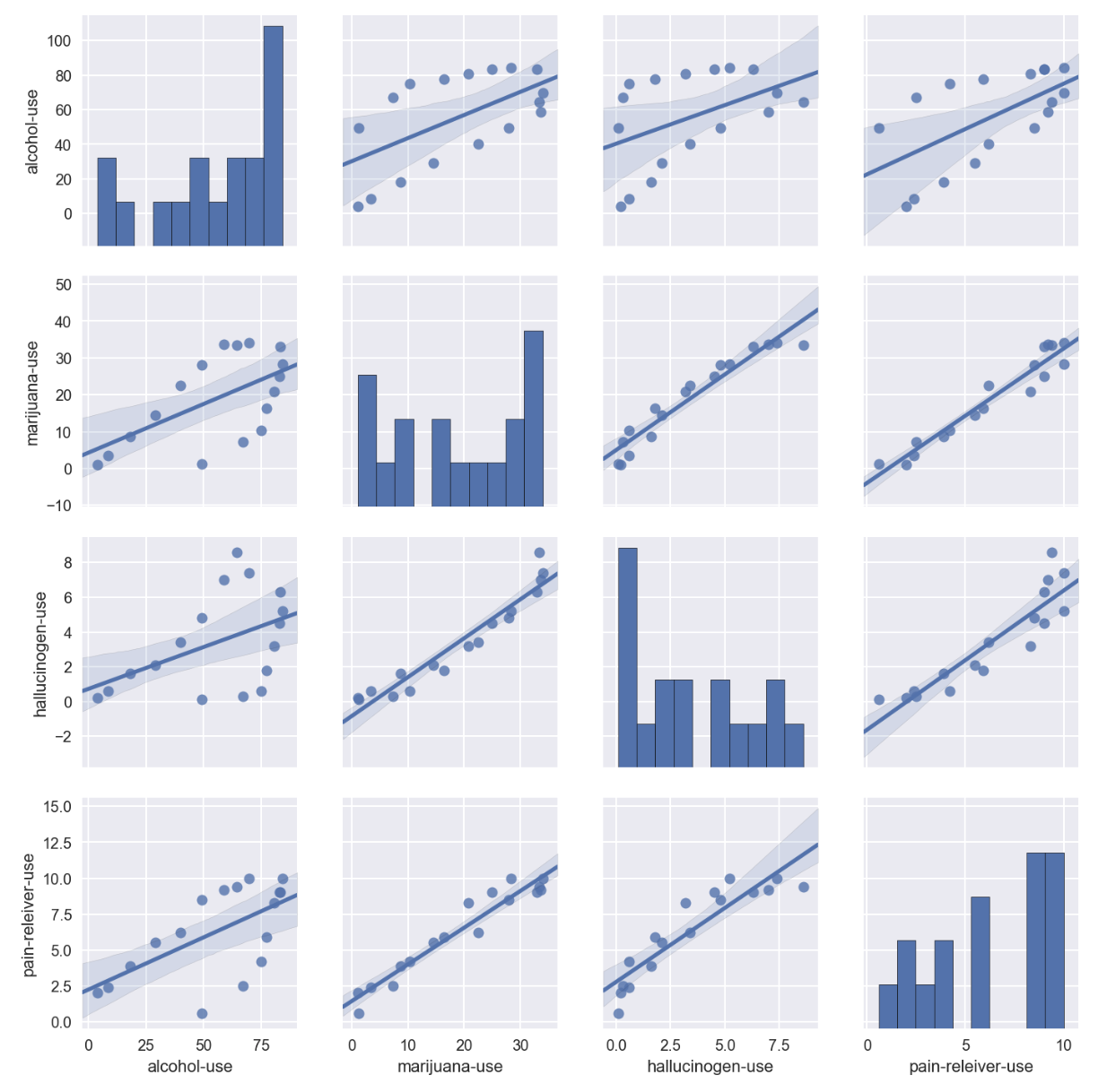
- all 4 drugs showed positive correlation to each other
- alcohol-use data was observed to behave more scatter-correlated with other drugs
- whilst the other 3 drugs(marijuana, hallucinogen, and pain-reliever) were found quite well positively correlated
2.7b : Check the correlation of data in drugFrequency dataset
plt.figure(figsize=(12,8))
sns.heatmap(data=drugFrequency_temp.corr(), cmap='RdBu_r', annot=True)
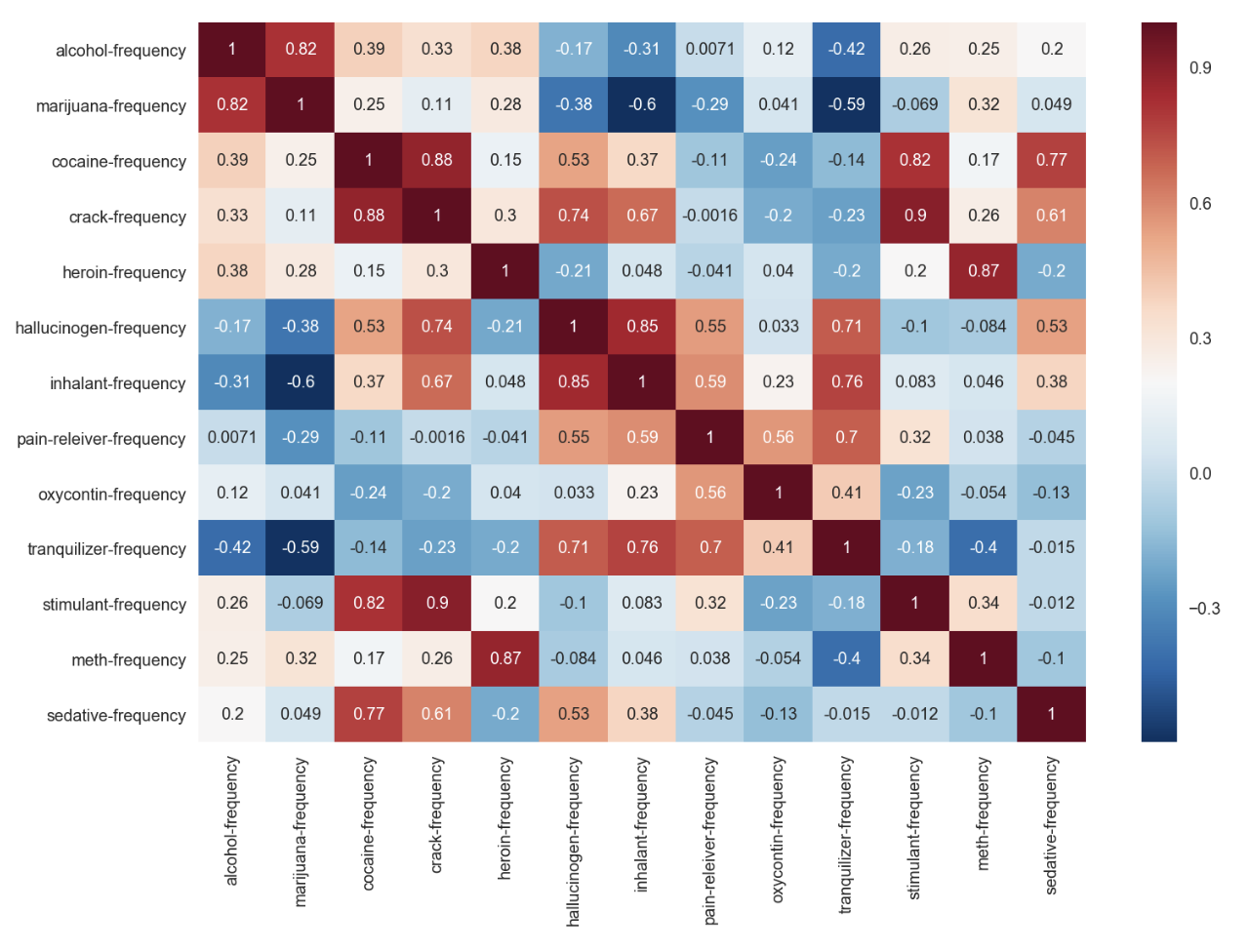
- mixture of positive and negative correlation among various drugFrequency
- crack-frequeny and stimulant-frequency has upto 0.9 positive correlation
Visualization the correlation of top 4 popular drugFreq(alcohol, marijuana, hallucinogen, and pain-reliever)
sns.pairplot(drugFrequency_temp[['alcohol-frequency','marijuana-frequency','hallucinogen-frequency','pain-releiver-frequency']],kind='reg')
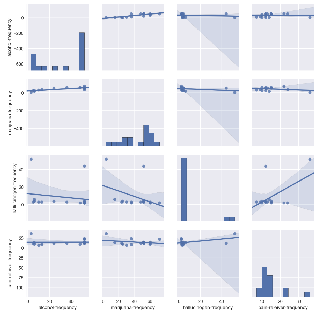
- No significant correlation was observed for all the 4 drugs frequency
- Hallucinogen-frequency was found having 2 extreme scale with majority of data at lower frequency level.
- The high hallucinogen-frequency data points could be outliers/exceptional intakes
Part 3 : Hypothesis Generation and Testing
In the data exploration process, it is common that we would need to generate some assumptions, testify and validate those assumptions before we can summarize the findings in order to make solid conclusions. For this session, observation in Part 2 was used to practise hypothesis generation and testing.
Question to explore :
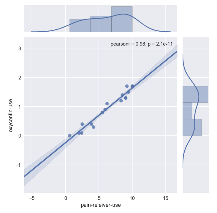
- Correlation matrix showed significant correlation (0.98) of oxycontin-use vs pain-reliever-use.
- Are the drug users in pain-reliever having the similar age group distribution as the drug users in oxycontine?
- \[H_0: Use_{pain-reliever} = Use_{oxycontin}\]
- \[H_1: Use_{pain-reliever} \neq Use_{oxycontin}\]
- But for their frequencies, correlation was only at 0.56. Are these correlation statistically significant?
- Among these 2 groups of drug users, are they taking the pain-reliever as frequent as oxycontine?
- \[H_0: frequency_{pain-reliever} = frequency_{oxycontin}\]
- \[H_1: frequency_{pain-reliever} \neq frequency_{oxycontin}\]
Deliverables :
- join-plot
- stats summary to include p-values
3.a : Comparison on Drug Use
1st examination through graphical view
sns.jointplot(x='pain-releiver-use', y='oxycontin-use', data=drugUse_temp, kind='reg')
2nd examination through stats library on p-value
p_value_drugUse = stats.ttest_ind(drugUse_temp['pain-releiver-use'],drugUse_temp['oxycontin-use'])
p_value_drugUse
Ttest_indResult(statistic=6.82263516475104, pvalue=1.0265878201430413e-07)
3.b : Comparison on Drug Frequency
1st examination through graphical view
- Repeat the same workflow as in 3.a
sns.jointplot(x='pain-releiver-frequency', y='oxycontin-frequency', data=drugFrequency_temp, kind='reg')
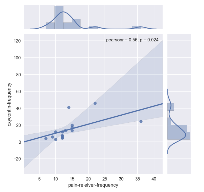
p_value_drugFrequency = stats.ttest_ind(drugFrequency_temp['pain-releiver-frequency'], drugFrequency_temp['oxycontin-frequency'],nan_policy='omit')
p_value_drugFrequency
# need to set nan_policy='omit' in order to ignore nan value in oxycontin-frequency for p-value calculation
Ttest_indResult(statistic=-0.030003630957118617, pvalue=0.9762564938195634)
Conclusion :
for drug use
Pearson correlation coefficient was close to 1, reported high at 0.98. p-value is small at 1.0265878201430413e-07, therefore null hypothesis is rejected drug user age group in pain-reliever is positively correlated to the drug user age group in oxycontine
for drug frequency
Pearson correlation coefficient was only at 0.56 p-value is small at 0.9762564938195634, therefore null hypothesis is accepted No conclusion can be made for drug frequency in pain reliever vs drug frequency in osycontine
Part 4 : Outliers Handling
Outliers handling is common in data analysis. In this session, a subset of the data is extracted and used to outline the flow on how outliers could be examined and corrected.
- Pain-reliever-frequency is used to study outlier effect
fig, ax = plt.subplots(2,1,figsize=(10,6), sharex=True)

sns.boxplot(data=drugFrequency_temp['pain-releiver-frequency'], orient='h',ax=ax[0])
sns.distplot(drugFrequency_temp['pain-releiver-frequency'], bins=30, ax=ax[1])
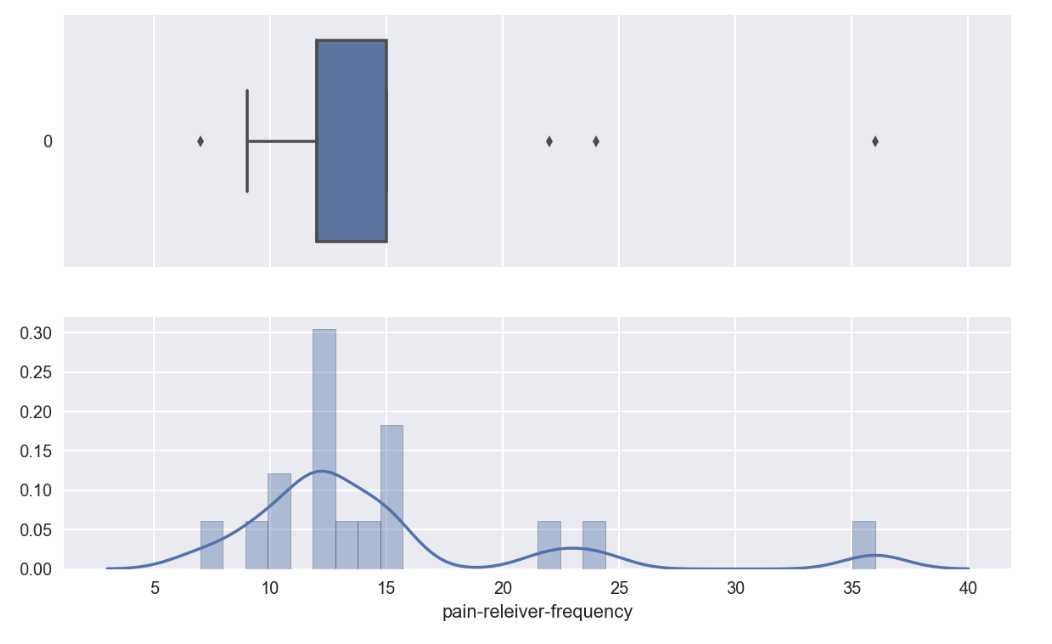
4 outlier data points were observed
4.a : Extraction of outlier data points
# Get the IQR
dataExamined = drugFrequency_temp['pain-releiver-frequency']
q25, q75 = np.percentile(dataExamined, [25,75])
IQR = q75 - q25

# Get outlier point below q25 and above q75
outliers_abv = dataExamined[dataExamined>(q75+1.5*IQR)]
outliers_below = dataExamined[dataExamined<(q25-1.5*IQR)]

# List out all outlier points
outliers_list = list(outliers_below.append(outliers_abv))
outliers_list
[7.0, 36.0, 22.0, 24.0]
4.b : Removal of outlier data points from examined dataset
dataExamined_clean = [v for v in dataExamined if v not in outliers_list]
print(len(dataExamined_clean))
dataExamined_clean
13


[14.0, 12.0, 10.0, 9.0, 12.0, 12.0, 10.0, 15.0, 15.0, 15.0, 13.0, 12.0, 12.0]
4.c : Comparison of mean, median, std dev for dataset with outliers vs no outlier
# set up dataframe for comparison
df_comparison = pd.DataFrame(dataExamined)
df_comparison.columns = ['With outliers']

# replace those identified as outlier point with nan in order to do stats calculation for scenario with no outliers
df_comparison['No outliers'] = df_comparison['With outliers'].map(lambda x: np.nan if x in outliers_list else x)
df_comparison.head()
| With outliers | No outliers | |
|---|---|---|
| 0 | 36.0 | NaN |
| 1 | 14.0 | 14.0 |
| 2 | 12.0 | 12.0 |
| 3 | 10.0 | 10.0 |
| 4 | 7.0 | NaN |
4.d : Tranpose dataframe for ease of comparison and calculation by columns
df_comparison_T = df_comparison.T
df_comparison_T
| 0 | 1 | 2 | 3 | 4 | 5 | 6 | 7 | 8 | 9 | 10 | 11 | 12 | 13 | 14 | 15 | 16 | |
|---|---|---|---|---|---|---|---|---|---|---|---|---|---|---|---|---|---|
| With outliers | 36.0 | 14.0 | 12.0 | 10.0 | 7.0 | 9.0 | 12.0 | 12.0 | 10.0 | 15.0 | 15.0 | 15.0 | 13.0 | 22.0 | 12.0 | 12.0 | 24.0 |
| No outliers | NaN | 14.0 | 12.0 | 10.0 | NaN | 9.0 | 12.0 | 12.0 | 10.0 | 15.0 | 15.0 | 15.0 | 13.0 | NaN | 12.0 | 12.0 | NaN |
df_comparison_T['mean'] = df_comparison_T.mean(axis=1)
df_comparison_T['median'] = df_comparison_T.median(axis=1)
df_comparison_T['stdDev'] = df_comparison_T.std(axis=1)
df_comparison_T
| 0 | 1 | 2 | 3 | 4 | 5 | 6 | 7 | 8 | 9 | 10 | 11 | 12 | 13 | 14 | 15 | 16 | mean | median | stdDev | |
|---|---|---|---|---|---|---|---|---|---|---|---|---|---|---|---|---|---|---|---|---|
| With outliers | 36.0 | 14.0 | 12.0 | 10.0 | 7.0 | 9.0 | 12.0 | 12.0 | 10.0 | 15.0 | 15.0 | 15.0 | 13.0 | 22.0 | 12.0 | 12.0 | 24.0 | 14.705882 | 12.5 | 6.558028 |
| No outliers | NaN | 14.0 | 12.0 | 10.0 | NaN | 9.0 | 12.0 | 12.0 | 10.0 | 15.0 | 15.0 | 15.0 | 13.0 | NaN | 12.0 | 12.0 | NaN | 12.384615 | 12.0 | 1.836437 |
df_comparison_T[['mean','median','stdDev']]
| mean | median | stdDev | |
|---|---|---|---|
| With outliers | 14.705882 | 12.5 | 6.558028 |
| No outliers | 12.384615 | 12.0 | 1.836437 |
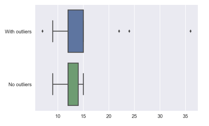
- all the 3 mean, median and stdDev are smaller when the outlier data points are excluded
sns.boxplot(data=df_comparison,orient='h')
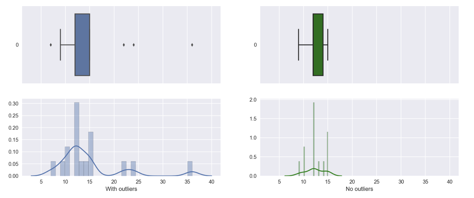
# addition plot to see the distribution of df with no outliers

fig, ax = plt.subplots(2,2,figsize=(15,6), sharex=True)

sns.boxplot(data=df_comparison['With outliers'], orient='h', ax=ax[0][0])
sns.distplot(df_comparison['With outliers'], bins=30, ax=ax[1][0])

sns.boxplot(data=df_comparison['No outliers'], orient='h', ax=ax[0][1], color='g')
sns.distplot(df_comparison.dropna()['No outliers'], bins=30, ax=ax[1][1], color='g')
Key Learnings
There are many techniques that we can use to explore data. No one single best method to outline how to explore the data perfectly. It is very much data dependent and can have different creative thoughts to present and visualize the data. Most importantly, the presented method is able to level up the understanding of the data and therefore expand the usage of such data for higher order of processing or modeling.