![]()
This project utilized an existing dataset ( Ames Housing Data @ Kaggle ) to predict the residential house prices. Through this project, algorithm was developed to reliably estimate the value of residential houses based on fixed features. Characteristics of the houses that the company could cost-effectively change/renovate were identified. Dataset was cleaned and analyzed thoroughly with comprehensive feature engineering. Model was then trained on pre-2010 data and tested its performance using 2010 housing data. The final model performance was characterized and the key features affecting the price were assessed and compared.
The project was splitted into 2 main parts
Part 1 : Estimating the value of homes from fixed characteristics
- Fixed characteristics refer to features that would involve major construction of the house
Part 2 : Determine any value of changeable property characteristics unexplained by the fixed ones.
- The effects in dollars of the renovate-able features were evaluated. By using the model obtained in Part 1, a review of its appropriateness to be used to assist the decision making if to buy/invest in the property was assessed. The variance in price remaining explainable by those features was therefore used as an indicator to justify such investment potentials.
Part 1 :
Estimating the Value of Houses from Fixed Characteristics
1.1 Data Preparation & Cleaning
- Filter raw dataset to have only residential related data
residential = house[house['MSZoning'] !='C (all)']

// quick graphical view to check columns with missing values
fig = plt.figure(figsize=(20,10))
sns.heatmap(residential.isnull(), cmap='viridis', cbar=False, yticklabels=False)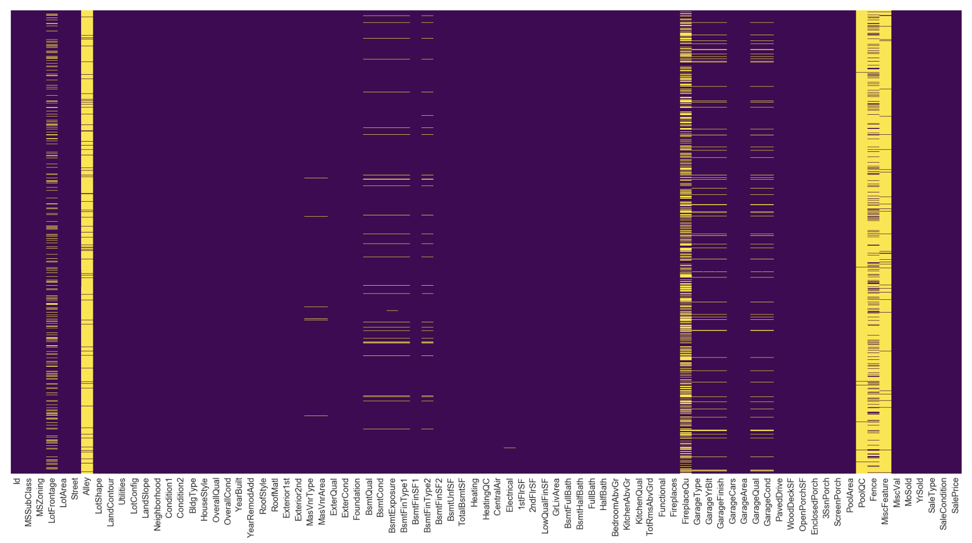
Percentage of missing values for affected columns was calculated and tabulated as below:
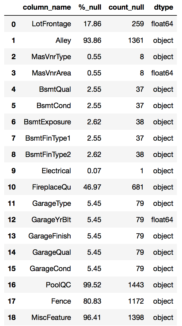
Columns with >45% missing values would be dropped in view of any replacement values would be assumption that impacted the accuracy significantly
Statistic of the remaining columns was reviewed in order to decide the best estimated values for those Na values. The review outcomes lead to the following decisions:
- for LotFrontage : mean and median were both at ~same value, the missing value to be replaced using median value
- for MasVnrArea : since there was only 8 Na and 50% of data is at 0, missing value to be replaced with median value of 0
- for MasVnrType : missing values were found corresponding to MasVnrArea. Since majority of data is None and MasVrnArea at 0, missing value to be replaced as None type
- for Bsmt related columns : data dictionary showed NA as No Basement. Further confirmation showed corresponding numerical columns with with Bsmt 0, missing value to be replaced with NA type
- for Electrical : since majority was under SBrkr, missing value to be replaced as SBrkr. This wouldn’t affect the overall distribution
- for Garage related columns : data dictionary showed NA as No Garage. Further confirmation showed corresponding numerical columns with Garage 0 or Na, missing value to be replaced with NA type and GarageYrBlt as 0
After imputation had been done, verification was carried out to check if there was any escapee during the replacement process
// final verification if anymore missing values

fig = plt.figure(figsize=(20,10))
sns.heatmap(residential.isnull(),cbar=False, yticklabels=False, cmap='viridis')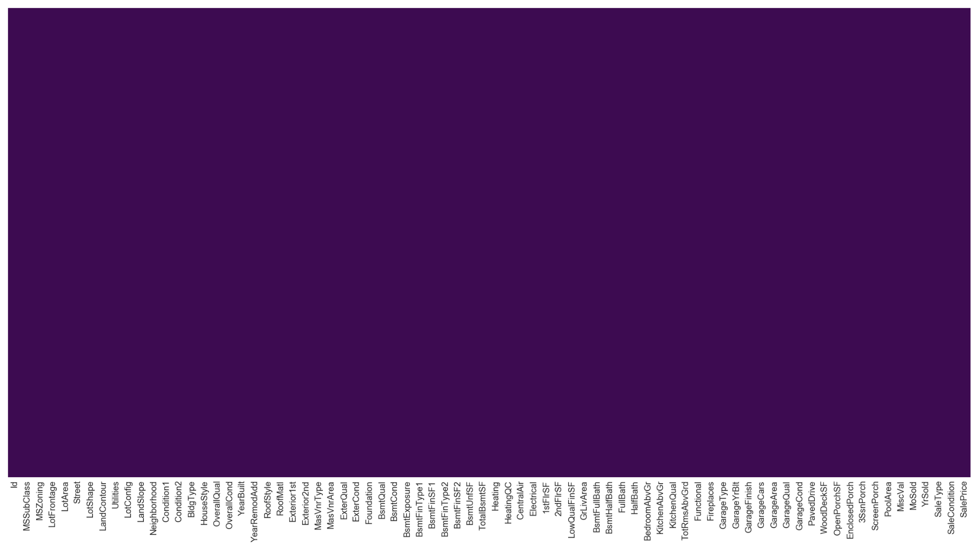
Result showed no more missing value. Data set was clean for further analysis.
1.2 : Identify fixed features for analysis
Fixed features refer to those features of the house that would involve major construction. The final fixed features were screened as below :
fixed_features = data_fix.columns
fixed_features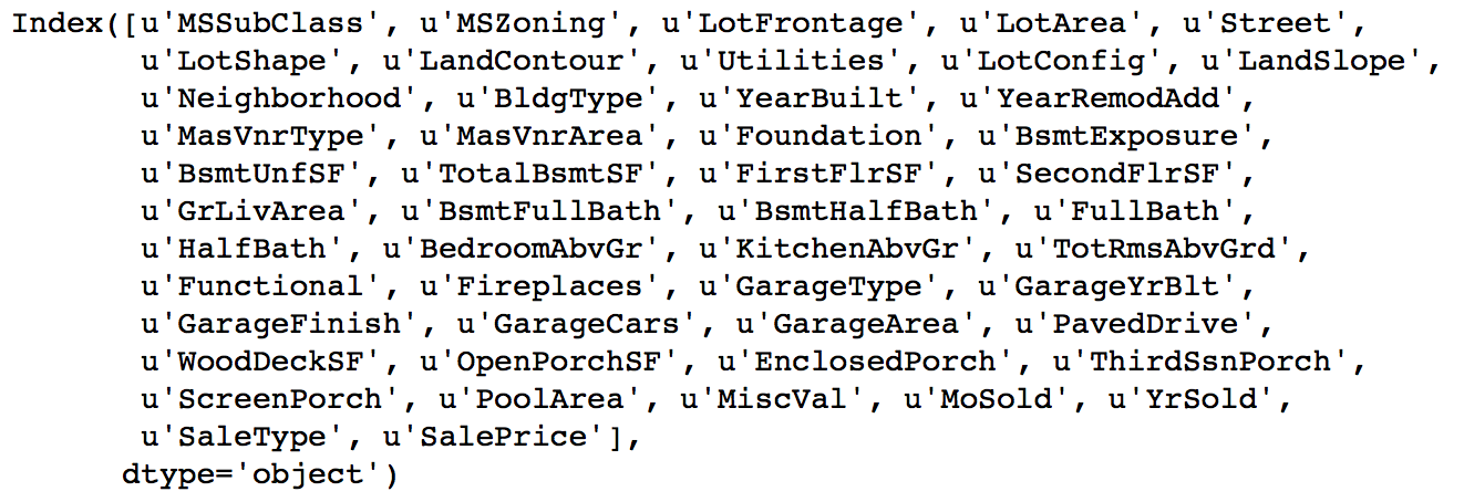
1.3 : Exploratory Data Analysis
// plot heatmap to check correlation

data_corr = data_fix.corr()
// Set the default matplotlib figure size:
fig, ax = plt.subplots(figsize=(15, 10))
// Generate a mask for the upper triangle (taken from seaborn example gallery)
mask = np.zeros_like(data_corr, dtype=np.bool)
mask[np.triu_indices_from(mask)] = True
// Plot the heatmap with seaborn.
// Assign the matplotlib axis the function returns. This will let us resize the labels.
ax = sns.heatmap(data_corr, mask=mask, ax=ax, cmap='Blues')
// Resize the labels.
ax.set_xticklabels(ax.xaxis.get_ticklabels(), fontsize=14)
ax.set_yticklabels(ax.yaxis.get_ticklabels(), fontsize=14)
plt.show()
// sns.heatmap(residential.corr(),cmap='Blues')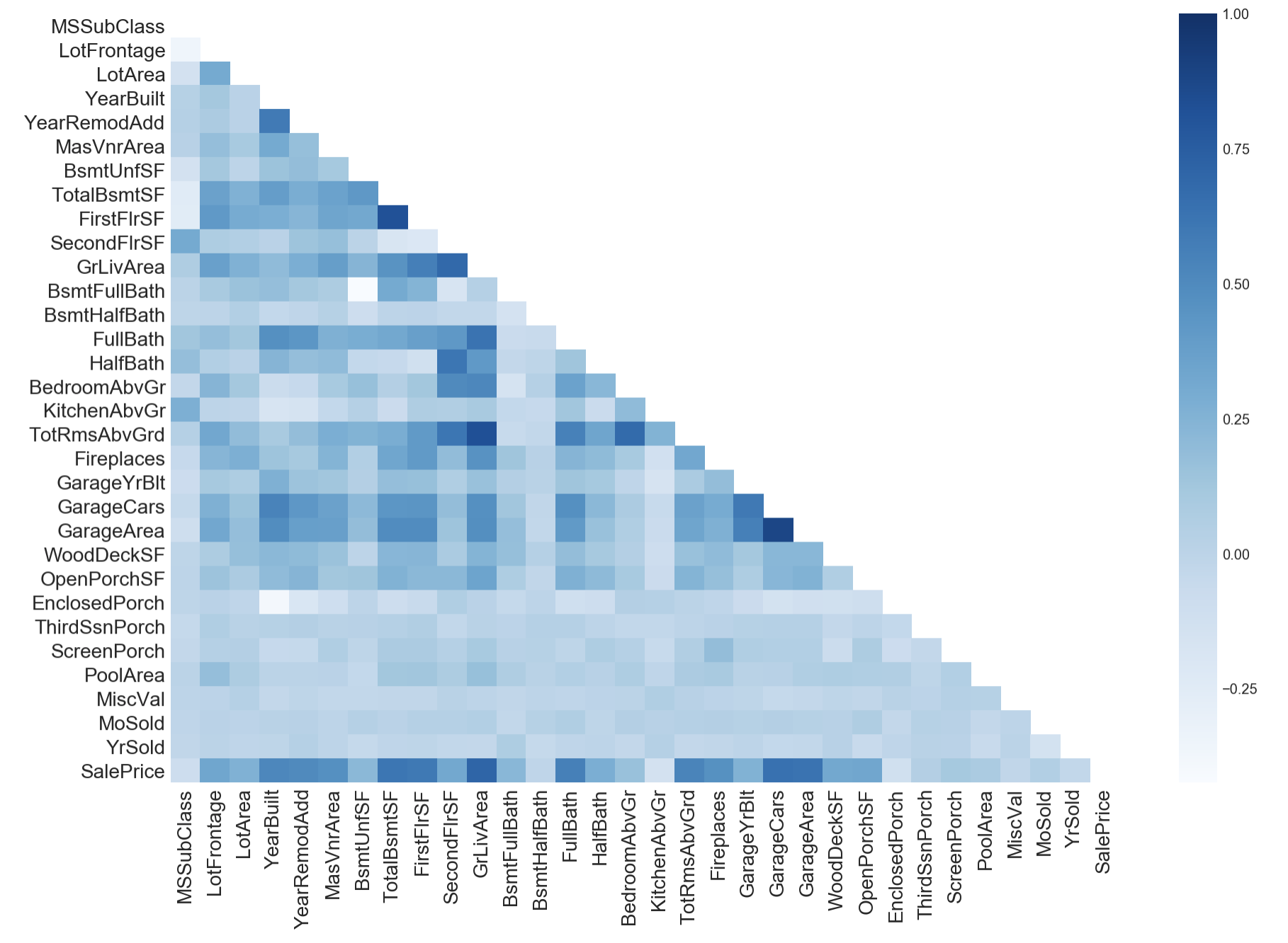
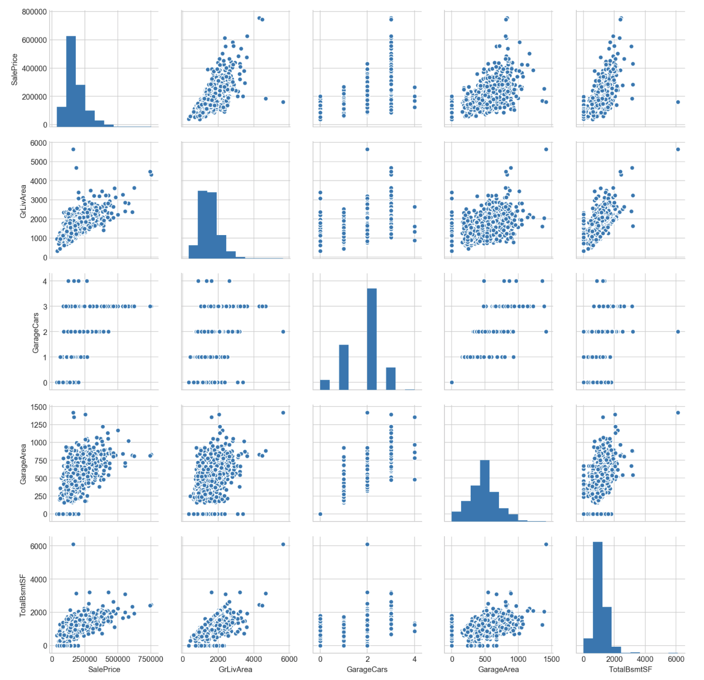
Visualization of the top 5 highly correlated variables :
1.4 : Modeling
// convert to matrices to prepare training data set with Patsy function

import patsy
y_fix, X_fix = patsy.dmatrices(formula, data=data_fix, return_type='dataframe')
// to confirm all categorical columns have been transformed with Patcy function above
X_fix.head()| MSZoning[T.RH] | MSZoning[T.RL] | MSZoning[T.RM] | Street[T.Pave] | LotShape[T.IR2] | LotShape[T.IR3] | LotShape[T.Reg] | LandContour[T.HLS] | LandContour[T.Low] | LandContour[T.Lvl] | Utilities[T.NoSeWa] | LotConfig[T.CulDSac] | LotConfig[T.FR2] | LotConfig[T.FR3] | LotConfig[T.Inside] | LandSlope[T.Mod] | LandSlope[T.Sev] | Neighborhood[T.Blueste] | Neighborhood[T.BrDale] | Neighborhood[T.BrkSide] | Neighborhood[T.ClearCr] | Neighborhood[T.CollgCr] | Neighborhood[T.Crawfor] | Neighborhood[T.Edwards] | Neighborhood[T.Gilbert] | Neighborhood[T.IDOTRR] | Neighborhood[T.MeadowV] | Neighborhood[T.Mitchel] | Neighborhood[T.NAmes] | Neighborhood[T.NPkVill] | Neighborhood[T.NWAmes] | Neighborhood[T.NoRidge] | Neighborhood[T.NridgHt] | Neighborhood[T.OldTown] | Neighborhood[T.SWISU] | Neighborhood[T.Sawyer] | Neighborhood[T.SawyerW] | Neighborhood[T.Somerst] | Neighborhood[T.StoneBr] | Neighborhood[T.Timber] | Neighborhood[T.Veenker] | BldgType[T.2fmCon] | BldgType[T.Duplex] | BldgType[T.Twnhs] | BldgType[T.TwnhsE] | MasVnrType[T.BrkFace] | MasVnrType[T.None] | MasVnrType[T.Stone] | Foundation[T.CBlock] | Foundation[T.PConc] | Foundation[T.Slab] | Foundation[T.Stone] | Foundation[T.Wood] | BsmtExposure[T.Gd] | BsmtExposure[T.Mn] | BsmtExposure[T.NA] | BsmtExposure[T.No] | Functional[T.Maj2] | Functional[T.Min1] | Functional[T.Min2] | Functional[T.Mod] | Functional[T.Sev] | Functional[T.Typ] | GarageType[T.Attchd] | GarageType[T.Basment] | GarageType[T.BuiltIn] | GarageType[T.CarPort] | GarageType[T.Detchd] | GarageType[T.NA] | GarageFinish[T.NA] | GarageFinish[T.RFn] | GarageFinish[T.Unf] | PavedDrive[T.P] | PavedDrive[T.Y] | SaleType[T.CWD] | SaleType[T.Con] | SaleType[T.ConLD] | SaleType[T.ConLI] | SaleType[T.ConLw] | SaleType[T.New] | SaleType[T.Oth] | SaleType[T.WD] | MSSubClass | LotFrontage | LotArea | YearBuilt | YearRemodAdd | MasVnrArea | BsmtUnfSF | TotalBsmtSF | FirstFlrSF | SecondFlrSF | GrLivArea | BsmtFullBath | BsmtHalfBath | FullBath | HalfBath | BedroomAbvGr | KitchenAbvGr | TotRmsAbvGrd | Fireplaces | GarageYrBlt | GarageCars | GarageArea | WoodDeckSF | OpenPorchSF | EnclosedPorch | ThirdSsnPorch | ScreenPorch | PoolArea | MiscVal | MoSold | YrSold | SalePrice | |
|---|---|---|---|---|---|---|---|---|---|---|---|---|---|---|---|---|---|---|---|---|---|---|---|---|---|---|---|---|---|---|---|---|---|---|---|---|---|---|---|---|---|---|---|---|---|---|---|---|---|---|---|---|---|---|---|---|---|---|---|---|---|---|---|---|---|---|---|---|---|---|---|---|---|---|---|---|---|---|---|---|---|---|---|---|---|---|---|---|---|---|---|---|---|---|---|---|---|---|---|---|---|---|---|---|---|---|---|---|---|---|---|---|---|---|
| 0 | 0.0 | 1.0 | 0.0 | 1.0 | 0.0 | 0.0 | 1.0 | 0.0 | 0.0 | 1.0 | 0.0 | 0.0 | 0.0 | 0.0 | 1.0 | 0.0 | 0.0 | 0.0 | 0.0 | 0.0 | 0.0 | 1.0 | 0.0 | 0.0 | 0.0 | 0.0 | 0.0 | 0.0 | 0.0 | 0.0 | 0.0 | 0.0 | 0.0 | 0.0 | 0.0 | 0.0 | 0.0 | 0.0 | 0.0 | 0.0 | 0.0 | 0.0 | 0.0 | 0.0 | 0.0 | 1.0 | 0.0 | 0.0 | 0.0 | 1.0 | 0.0 | 0.0 | 0.0 | 0.0 | 0.0 | 0.0 | 1.0 | 0.0 | 0.0 | 0.0 | 0.0 | 0.0 | 1.0 | 1.0 | 0.0 | 0.0 | 0.0 | 0.0 | 0.0 | 0.0 | 1.0 | 0.0 | 0.0 | 1.0 | 0.0 | 0.0 | 0.0 | 0.0 | 0.0 | 0.0 | 0.0 | 1.0 | 60.0 | 65.0 | 8450.0 | 2003.0 | 2003.0 | 196.0 | 150.0 | 856.0 | 856.0 | 854.0 | 1710.0 | 1.0 | 0.0 | 2.0 | 1.0 | 3.0 | 1.0 | 8.0 | 0.0 | 2003.0 | 2.0 | 548.0 | 0.0 | 61.0 | 0.0 | 0.0 | 0.0 | 0.0 | 0.0 | 2.0 | 2008.0 | 208500.0 |
| 1 | 0.0 | 1.0 | 0.0 | 1.0 | 0.0 | 0.0 | 1.0 | 0.0 | 0.0 | 1.0 | 0.0 | 0.0 | 1.0 | 0.0 | 0.0 | 0.0 | 0.0 | 0.0 | 0.0 | 0.0 | 0.0 | 0.0 | 0.0 | 0.0 | 0.0 | 0.0 | 0.0 | 0.0 | 0.0 | 0.0 | 0.0 | 0.0 | 0.0 | 0.0 | 0.0 | 0.0 | 0.0 | 0.0 | 0.0 | 0.0 | 1.0 | 0.0 | 0.0 | 0.0 | 0.0 | 0.0 | 1.0 | 0.0 | 1.0 | 0.0 | 0.0 | 0.0 | 0.0 | 1.0 | 0.0 | 0.0 | 0.0 | 0.0 | 0.0 | 0.0 | 0.0 | 0.0 | 1.0 | 1.0 | 0.0 | 0.0 | 0.0 | 0.0 | 0.0 | 0.0 | 1.0 | 0.0 | 0.0 | 1.0 | 0.0 | 0.0 | 0.0 | 0.0 | 0.0 | 0.0 | 0.0 | 1.0 | 20.0 | 80.0 | 9600.0 | 1976.0 | 1976.0 | 0.0 | 284.0 | 1262.0 | 1262.0 | 0.0 | 1262.0 | 0.0 | 1.0 | 2.0 | 0.0 | 3.0 | 1.0 | 6.0 | 1.0 | 1976.0 | 2.0 | 460.0 | 298.0 | 0.0 | 0.0 | 0.0 | 0.0 | 0.0 | 0.0 | 5.0 | 2007.0 | 181500.0 |
| 2 | 0.0 | 1.0 | 0.0 | 1.0 | 0.0 | 0.0 | 0.0 | 0.0 | 0.0 | 1.0 | 0.0 | 0.0 | 0.0 | 0.0 | 1.0 | 0.0 | 0.0 | 0.0 | 0.0 | 0.0 | 0.0 | 1.0 | 0.0 | 0.0 | 0.0 | 0.0 | 0.0 | 0.0 | 0.0 | 0.0 | 0.0 | 0.0 | 0.0 | 0.0 | 0.0 | 0.0 | 0.0 | 0.0 | 0.0 | 0.0 | 0.0 | 0.0 | 0.0 | 0.0 | 0.0 | 1.0 | 0.0 | 0.0 | 0.0 | 1.0 | 0.0 | 0.0 | 0.0 | 0.0 | 1.0 | 0.0 | 0.0 | 0.0 | 0.0 | 0.0 | 0.0 | 0.0 | 1.0 | 1.0 | 0.0 | 0.0 | 0.0 | 0.0 | 0.0 | 0.0 | 1.0 | 0.0 | 0.0 | 1.0 | 0.0 | 0.0 | 0.0 | 0.0 | 0.0 | 0.0 | 0.0 | 1.0 | 60.0 | 68.0 | 11250.0 | 2001.0 | 2002.0 | 162.0 | 434.0 | 920.0 | 920.0 | 866.0 | 1786.0 | 1.0 | 0.0 | 2.0 | 1.0 | 3.0 | 1.0 | 6.0 | 1.0 | 2001.0 | 2.0 | 608.0 | 0.0 | 42.0 | 0.0 | 0.0 | 0.0 | 0.0 | 0.0 | 9.0 | 2008.0 | 223500.0 |
| 3 | 0.0 | 1.0 | 0.0 | 1.0 | 0.0 | 0.0 | 0.0 | 0.0 | 0.0 | 1.0 | 0.0 | 0.0 | 0.0 | 0.0 | 0.0 | 0.0 | 0.0 | 0.0 | 0.0 | 0.0 | 0.0 | 0.0 | 1.0 | 0.0 | 0.0 | 0.0 | 0.0 | 0.0 | 0.0 | 0.0 | 0.0 | 0.0 | 0.0 | 0.0 | 0.0 | 0.0 | 0.0 | 0.0 | 0.0 | 0.0 | 0.0 | 0.0 | 0.0 | 0.0 | 0.0 | 0.0 | 1.0 | 0.0 | 0.0 | 0.0 | 0.0 | 0.0 | 0.0 | 0.0 | 0.0 | 0.0 | 1.0 | 0.0 | 0.0 | 0.0 | 0.0 | 0.0 | 1.0 | 0.0 | 0.0 | 0.0 | 0.0 | 1.0 | 0.0 | 0.0 | 0.0 | 1.0 | 0.0 | 1.0 | 0.0 | 0.0 | 0.0 | 0.0 | 0.0 | 0.0 | 0.0 | 1.0 | 70.0 | 60.0 | 9550.0 | 1915.0 | 1970.0 | 0.0 | 540.0 | 756.0 | 961.0 | 756.0 | 1717.0 | 1.0 | 0.0 | 1.0 | 0.0 | 3.0 | 1.0 | 7.0 | 1.0 | 1998.0 | 3.0 | 642.0 | 0.0 | 35.0 | 272.0 | 0.0 | 0.0 | 0.0 | 0.0 | 2.0 | 2006.0 | 140000.0 |
| 4 | 0.0 | 1.0 | 0.0 | 1.0 | 0.0 | 0.0 | 0.0 | 0.0 | 0.0 | 1.0 | 0.0 | 0.0 | 1.0 | 0.0 | 0.0 | 0.0 | 0.0 | 0.0 | 0.0 | 0.0 | 0.0 | 0.0 | 0.0 | 0.0 | 0.0 | 0.0 | 0.0 | 0.0 | 0.0 | 0.0 | 0.0 | 1.0 | 0.0 | 0.0 | 0.0 | 0.0 | 0.0 | 0.0 | 0.0 | 0.0 | 0.0 | 0.0 | 0.0 | 0.0 | 0.0 | 1.0 | 0.0 | 0.0 | 0.0 | 1.0 | 0.0 | 0.0 | 0.0 | 0.0 | 0.0 | 0.0 | 0.0 | 0.0 | 0.0 | 0.0 | 0.0 | 0.0 | 1.0 | 1.0 | 0.0 | 0.0 | 0.0 | 0.0 | 0.0 | 0.0 | 1.0 | 0.0 | 0.0 | 1.0 | 0.0 | 0.0 | 0.0 | 0.0 | 0.0 | 0.0 | 0.0 | 1.0 | 60.0 | 84.0 | 14260.0 | 2000.0 | 2000.0 | 350.0 | 490.0 | 1145.0 | 1145.0 | 1053.0 | 2198.0 | 1.0 | 0.0 | 2.0 | 1.0 | 4.0 | 1.0 | 9.0 | 1.0 | 2000.0 | 3.0 | 836.0 | 192.0 | 84.0 | 0.0 | 0.0 | 0.0 | 0.0 | 0.0 | 12.0 | 2008.0 | 250000.0 |
// Split data to train set (before 2010) and test set ( after 2010)

X_fix_train = X_fix[X_fix['YrSold']<2010].drop('SalePrice', axis=1)
X_fix_test = X_fix[X_fix['YrSold']>=2010].drop('SalePrice', axis=1)

y_fix_train = X_fix[X_fix['YrSold']<2010]['SalePrice']
y_fix_test = X_fix[X_fix['YrSold']>=2010]['SalePrice']

// standardize the X variables:

Xs_fix_train = ss.fit_transform(X_fix_train)
Xs_fix_test = ss.fit_transform(X_fix_test)

// modeling with Lasso:

model_lasso.fit(Xs_fix_train, y_fix_train)
predicted_y_fix = model_lasso.predict(Xs_fix_test)

coefficient_fix = model_lasso.coef_
score_fix = model_lasso.score(Xs_fix_test, y_fix_test)
score_fix
'''
0.8803540439252586
'''Visualization of residual/gap of predicted vs actual sales price and their coefficient differences
residual_fix_data = pd.DataFrame(list(zip(y_fix_test, predicted_y_fix)), columns=['Actual SalePrice', 'Predicted SalePrice'])sns.lmplot(x='Actual SalePrice', y='Predicted SalePrice', data=residual_fix_data)
plt.title('Prediction of SalePrice with Fix features only')
plt.show()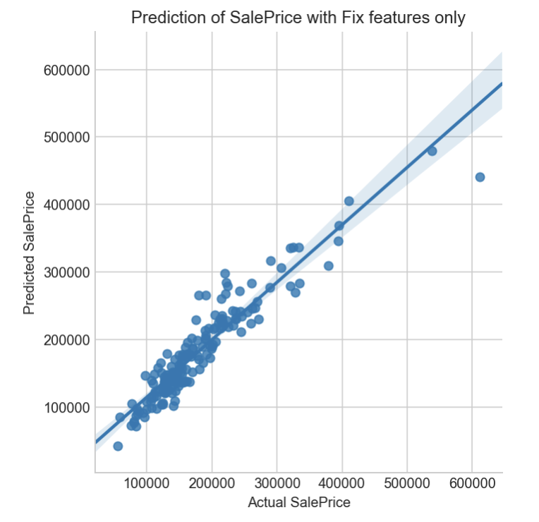
sns.residplot(x='Actual SalePrice', y='Predicted SalePrice', data=residual_fix_data)
plt.title('Residual Plot of SalePrice with Fix features only')
plt.show()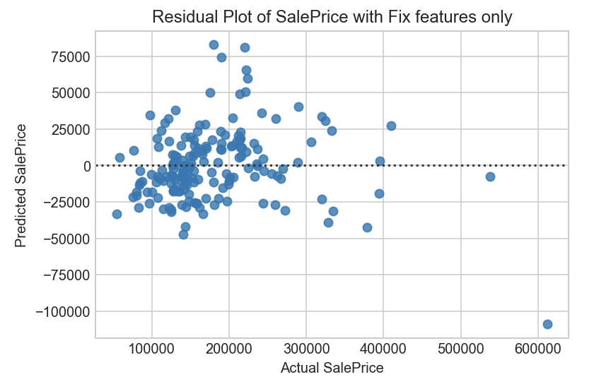
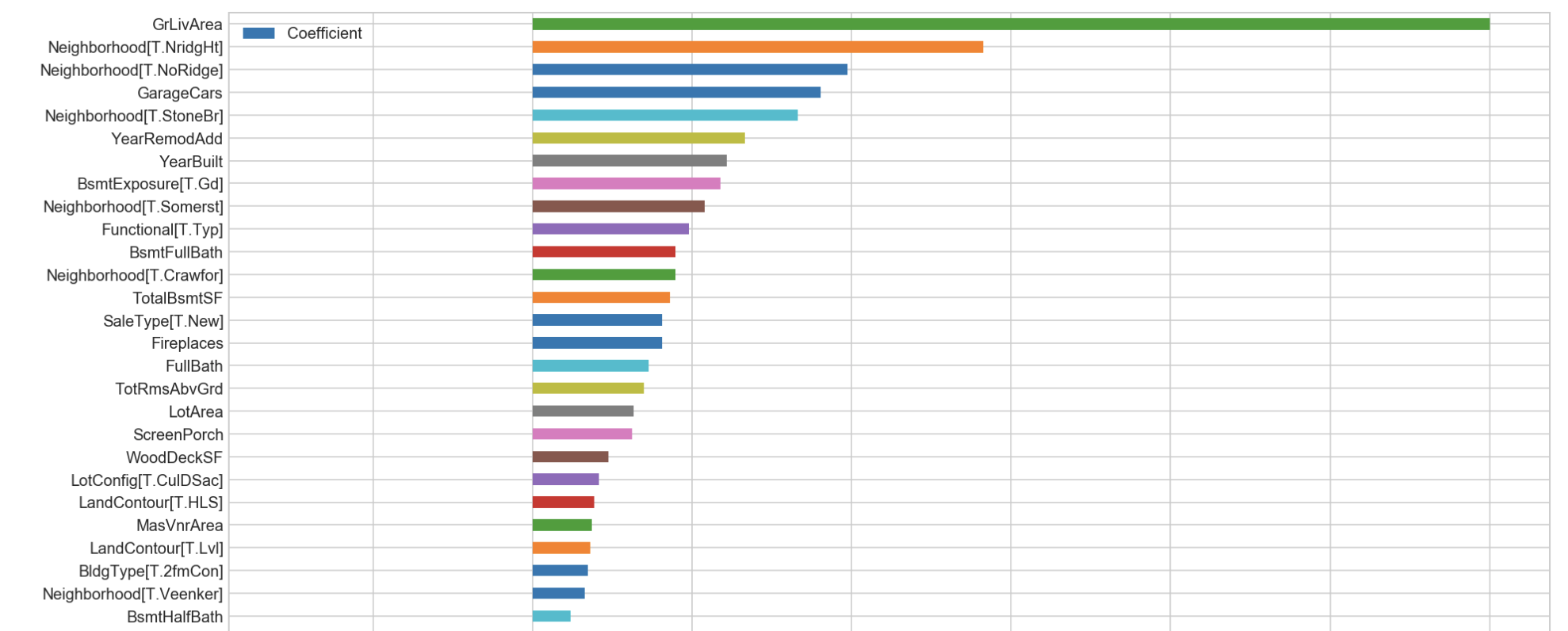
coefficient_fix_df = pd.DataFrame(list(zip(X_fix_test.columns, coefficient_fix)),columns=['Features','Coefficient'])
coefficient_fix_df.sort_values('Coefficient', ascending=True).plot(x='Features', y='Coefficient', kind='barh', figsize=(15,30))
plt.show()
Partial view of the coeefficient graph
no_of_variables_in_modeling2 = len(coefficient_fix_df[coefficient_fix_df.values != 0])
no_of_variables_in_modeling2

'''
186
'''
MAE_2 = mean_absolute_error(y_fix_test, predicted_y_fix)
MSE_2 = mean_squared_error(y_fix_test, predicted_y_fix)
RMSE_2 = np.sqrt(mean_squared_error(y_fix_test, predicted_y_fix))
print('MAE\t = {}'.format(MAE_2))
print('MSE\t = {}'.format(MSE_2))
print('RMSE\t = {}'.format(RMSE_2))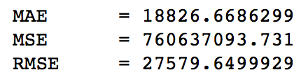
Part 2 :
Determine any value of changeable property characteristics unexplained by the fixed ones.
Workflow in P1 was repeated, but for part 2 all variables ( fix + nonfix ) were included into calculation.
For modeling, Grid Search on Lasso was used to assist finding the best parameters for price prediction.
from sklearn.model_selection import GridSearchCV
from sklearn.linear_model import Lasso

alphas = np.logspace(-5, 5, 20)

model_gs = GridSearchCV(estimator=Lasso(), param_grid=dict(alpha=alphas), cv=10, scoring='r2')
model_gs.fit(Xs_mix_train, y_mix_train)

model_gs.best_estimator_.score(Xs_mix_test, y_mix_test)

'''
0.886990270681429
'''
Model score was found very close to earlier score obtained in Part 1, indicating there could be little/no difference caused by renovation effect. Model using LassoCV was finalized and continued with the calculation on cost of renovation effects.
2.1 The effect in dollars of SalePrice with renovate-able features
Relevant information was tabulated to summarize the effect in dollars on SalePrice with renovatable features
cost_effect_comparison = merge_table_mix_fix[['Actual SalePrice_Mix','Predicted SalePrice_Mix','Predicted SalePrice_Fix']].copy()

// add new column to calculate cost of renovation effect:
cost_effect_comparison['Cost of Renovation Effect'] = merge_table_mix_fix['Predicted SalePrice_Mix'] - merge_table_mix_fix['Predicted SalePrice_Fix']

// add new column to calculate the % increase in predicted SalePrice factoring renovate-able features:
cost_effect_comparison['% of Increase due to Renovation'] = cost_effect_comparison['Cost of Renovation Effect']/cost_effect_comparison['Predicted SalePrice_Mix']*100

cost_effect_comparison.sort_values('% of Increase due to Renovation', ascending=False)

// cost of Reno effect = Predicted SalePrice_Mix - Predicted SalePrice_Fix
// Impact of reno effect is presented through % of Increase in SalePrice
Partial view of the tabulated cost of renovation effects :
| Actual SalePrice_Mix | Predicted SalePrice_Mix | Predicted SalePrice_Fix | Cost of Renovation Effect | % of Increase due to Renovation | |
|---|---|---|---|---|---|
| 84 | 55000.0 | 61664.957714 | 42891.117349 | 18773.840365 | 30.44 |
| 138 | 164000.0 | 237093.364080 | 179208.778886 | 57884.585194 | 24.41 |
| 77 | 88000.0 | 120260.063071 | 93523.405892 | 26736.657180 | 22.23 |
| 120 | 100000.0 | 122506.492606 | 96293.063784 | 26213.428821 | 21.40 |
| 99 | 155000.0 | 156570.449387 | 135831.029298 | 20739.420089 | 13.25 |
| 147 | 139000.0 | 138312.341658 | 120976.916906 | 17335.424753 | 12.53 |
// Visualize effect on SalePrice with renovate-able features
// Effect on each individual listing could therefore be identified visually

fig = plt.figure(figsize=(20,10))
sns.barplot(x=cost_effect_comparison.index, y=cost_effect_comparison['% of Increase due to Renovation'])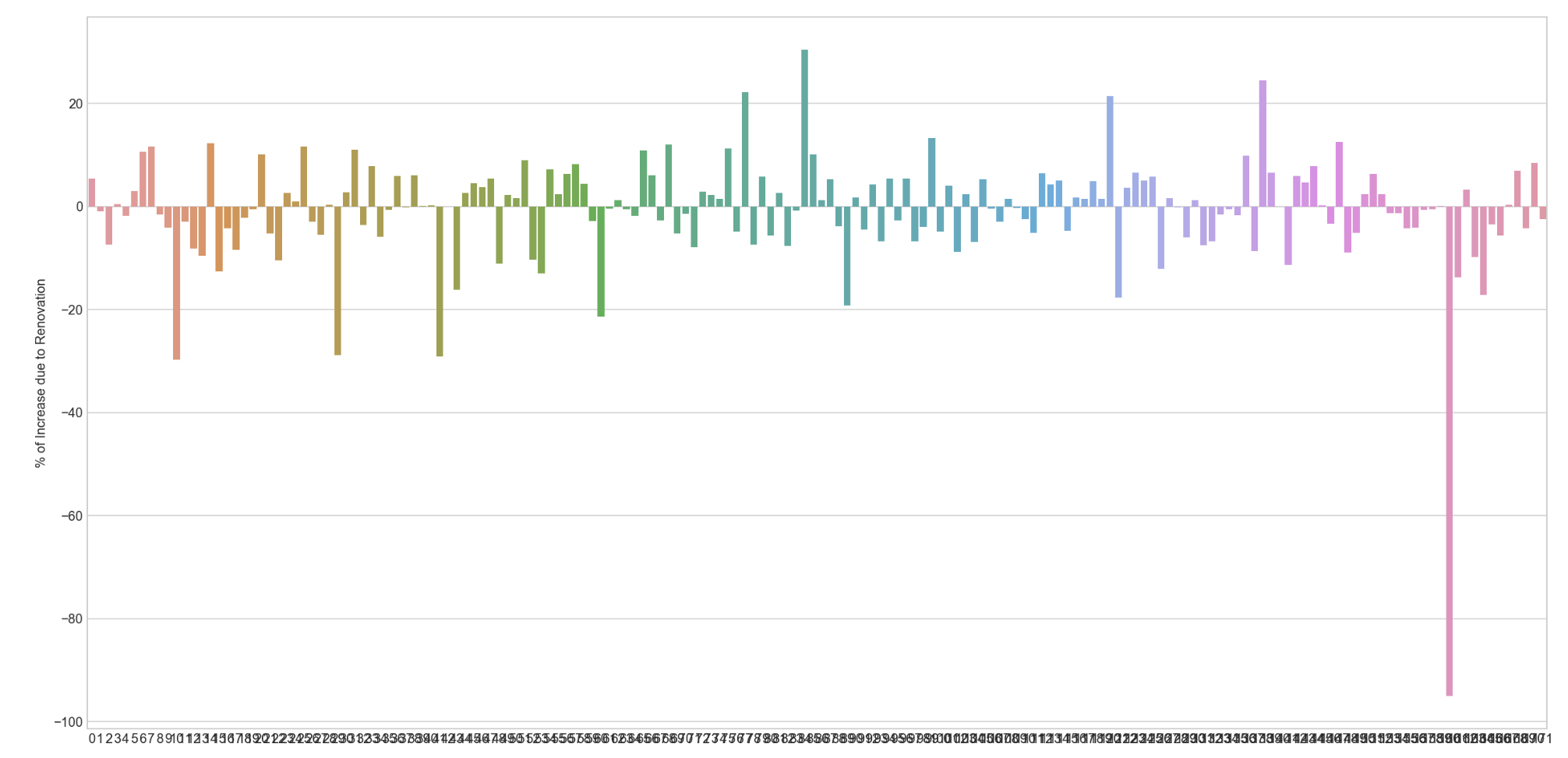
// distribution of the effect of renovate-able features on SalePrice:

fig = plt.figure(figsize=(15,7))
sns.distplot( cost_effect_comparison['% of Increase due to Renovation'])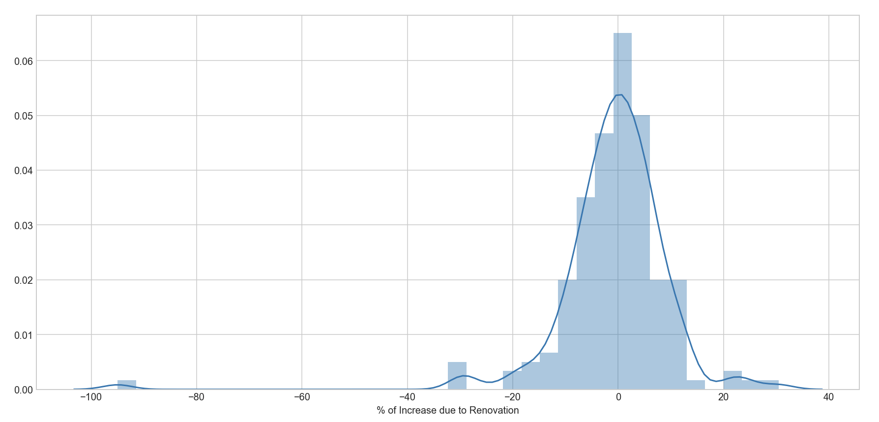
Outlier to the left( negative effect of renovate-able feature ) could be due to odd/non prime location in which original house condition is also possibly bad causing high renovation cost needed
// Check outlier unit to see if it is tally with the assumption

residential[residential.index == 160]| Id | MSSubClass | MSZoning | LotFrontage | LotArea | Street | LotShape | LandContour | Utilities | LotConfig | LandSlope | Neighborhood | Condition1 | Condition2 | BldgType | HouseStyle | OverallQual | OverallCond | YearBuilt | YearRemodAdd | RoofStyle | RoofMatl | Exterior1st | Exterior2nd | MasVnrType | MasVnrArea | ExterQual | ExterCond | Foundation | BsmtQual | BsmtCond | BsmtExposure | BsmtFinType1 | BsmtFinSF1 | BsmtFinType2 | BsmtFinSF2 | BsmtUnfSF | TotalBsmtSF | Heating | HeatingQC | CentralAir | Electrical | FirstFlrSF | SecondFlrSF | LowQualFinSF | GrLivArea | BsmtFullBath | BsmtHalfBath | FullBath | HalfBath | BedroomAbvGr | KitchenAbvGr | KitchenQual | TotRmsAbvGrd | Functional | Fireplaces | GarageType | GarageYrBlt | GarageFinish | GarageCars | GarageArea | GarageQual | GarageCond | PavedDrive | WoodDeckSF | OpenPorchSF | EnclosedPorch | ThirdSsnPorch | ScreenPorch | PoolArea | MiscVal | MoSold | YrSold | SaleType | SaleCondition | SalePrice | |
|---|---|---|---|---|---|---|---|---|---|---|---|---|---|---|---|---|---|---|---|---|---|---|---|---|---|---|---|---|---|---|---|---|---|---|---|---|---|---|---|---|---|---|---|---|---|---|---|---|---|---|---|---|---|---|---|---|---|---|---|---|---|---|---|---|---|---|---|---|---|---|---|---|---|---|---|---|
| 160 | 161 | 20 | RL | 70.0 | 11120 | Pave | IR1 | Lvl | AllPub | CulDSac | Gtl | Veenker | Norm | Norm | 1Fam | 1Story | 6 | 6 | 1984 | 1984 | Gable | CompShg | Plywood | Plywood | None | 0.0 | TA | TA | PConc | Gd | TA | No | BLQ | 660 | Unf | 0 | 572 | 1232 | GasA | TA | Y | SBrkr | 1232 | 0 | 0 | 1232 | 0 | 0 | 2 | 0 | 3 | 1 | TA | 6 | Typ | 0 | Attchd | 1984.0 | Unf | 2 | 516 | TA | TA | Y | 0 | 0 | 0 | 0 | 0 | 0 | 0 | 6 | 2008 | WD | Normal | 162500 |
From data dictionary, it was found that :
- 20 : 1-STORY 1946 & NEWER ALL STYLES => old house
- RL : Residential Low Density => non prime location
- IR1 : Slightly irregular => irregular lot size
- Lvl : Near Flat/Level
- CulDSac : Cul-de-sac
- Gtl : Gentle slope
- 1Fam : Single-family Detached
- OverallQual : 6 Above Average => quality is still within the mean quality level of majority
The closest explanation to the outlier point in which the unit had low predicted saleprice even after factoring renovate-able features was due to the house physical condition of being ancient old house with irregular size situated at non-prime location.
2.2 Use of Coefficients for Decision Making : To buy / Not to Buy
For ease of understanding, the coefficients were tabulated and visualized through graphical view
// visualize the coefficient :
coefficient_mix_df = pd.DataFrame(list(zip(X_mix_test.columns, coefficient_mix)),columns=['Features','Coefficient'])
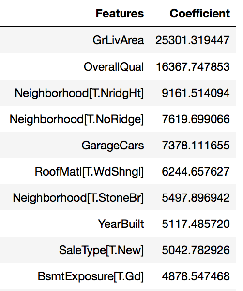
coefficient_mix_df.sort_values('Coefficient', ascending=False)Partial view of the tabulated coefficients as below :
// graphical view of coefficient differences :

// exclude features with 0 coeeficient value to be displayed on the chart
coefficient_plot = coefficient_mix_df[coefficient_mix_df['Coefficient']!=0]

coefficient_plot.sort_values('Coefficient', ascending=True).plot(x='Features', y='Coefficient', kind='barh', figsize=(15,30))
plt.show()
Partial view of the graphical representation of coefficients as below :
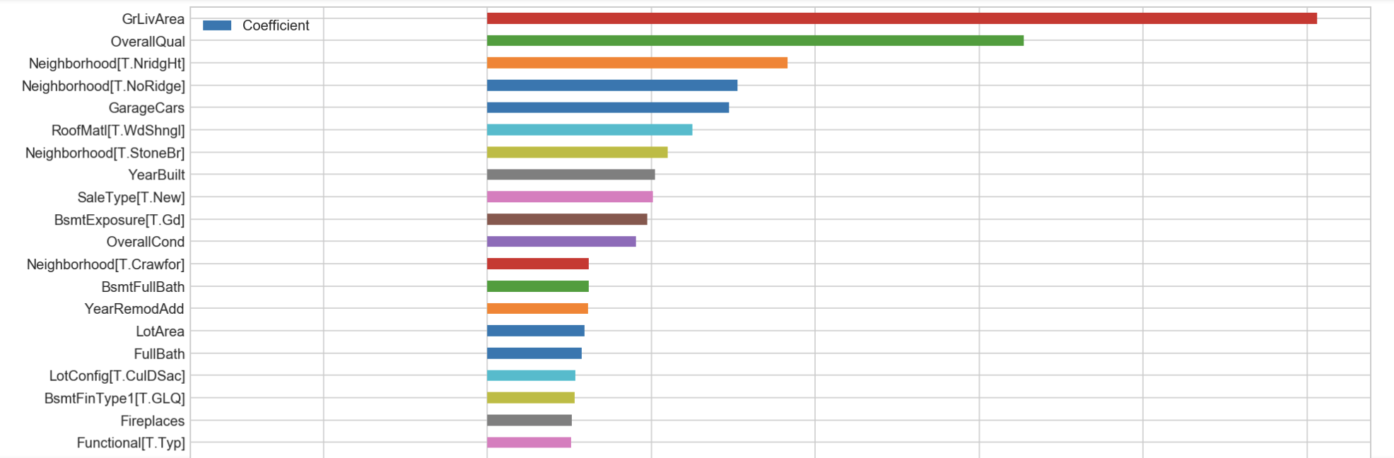
Top 3 highest coefficients could be used as estimators for higher achievable predicted saleprice
- GrLivArea: Above grade (ground) living area square feet
- OverallQual: Rates the overall material and finish of the house
- Neighborhood: Northridge Heights
2.3 Variance in Price Remaining Explainable by Features
[ Which renovate-able features are effective in increasing predicted SalePrice ]
To further identify & finalize real renovatable_features excluding physical conditions:
renovatable_features = ['Condition1[T.Feedr]','Condition1[T.Norm]','Condition1[T.PosA]','Condition1[T.PosN]','Condition1[T.RRAe]','Condition1[T.RRAn]','Condition1[T.RRNe]','Condition1[T.RRNn]','Condition2[T.Feedr]','Condition2[T.Norm]','Condition2[T.PosA]','Condition2[T.PosN]','Condition2[T.RRAe]','Condition2[T.RRAn]','Condition2[T.RRNn]','HouseStyle[T.1.5Unf]','HouseStyle[T.1Story]','HouseStyle[T.2.5Fin]','HouseStyle[T.2.5Unf]','HouseStyle[T.2Story]','HouseStyle[T.SFoyer]','HouseStyle[T.SLvl]','RoofStyle[T.Gable]','RoofStyle[T.Gambrel]','RoofStyle[T.Hip]','RoofStyle[T.Mansard]','RoofStyle[T.Shed]','RoofMatl[T.CompShg]','RoofMatl[T.Membran]','RoofMatl[T.Metal]','RoofMatl[T.Roll]','RoofMatl[T.Tar&Grv]','RoofMatl[T.WdShake]','RoofMatl[T.WdShngl]','Exterior1st[T.AsphShn]','Exterior1st[T.BrkComm]','Exterior1st[T.BrkFace]','Exterior1st[T.CBlock]','Exterior1st[T.CemntBd]','Exterior1st[T.HdBoard]','Exterior1st[T.ImStucc]','Exterior1st[T.MetalSd]','Exterior1st[T.Plywood]','Exterior1st[T.Stone]','Exterior1st[T.Stucco]','Exterior1st[T.VinylSd]','Exterior1st[T.WdSdng]','Exterior1st[T.WdShing]','Exterior2nd[T.AsphShn]','Exterior2nd[T.BrkCmn]','Exterior2nd[T.BrkFace]','Exterior2nd[T.CBlock]','Exterior2nd[T.CmentBd]','Exterior2nd[T.HdBoard]','Exterior2nd[T.ImStucc]','Exterior2nd[T.MetalSd]','Exterior2nd[T.Other]','Exterior2nd[T.Plywood]','Exterior2nd[T.Stone]','Exterior2nd[T.Stucco]','Exterior2nd[T.VinylSd]','Exterior2nd[T.WdSdng]','Exterior2nd[T.WdShng]','MasVnrType[T.BrkFace]','MasVnrType[T.None]','MasVnrType[T.Stone]','ExterQual[T.Fa]','ExterQual[T.Gd]','ExterQual[T.TA]','ExterCond[T.Fa]','ExterCond[T.Gd]','ExterCond[T.Po]','ExterCond[T.TA]','BsmtQual[T.Fa]','BsmtQual[T.Gd]','BsmtQual[T.NA]','BsmtQual[T.TA]','BsmtCond[T.Gd]','BsmtCond[T.NA]','BsmtCond[T.Po]','BsmtCond[T.TA]','BsmtExposure[T.Gd]','BsmtExposure[T.Mn]','BsmtExposure[T.NA]','BsmtExposure[T.No]','BsmtFinType1[T.BLQ]','BsmtFinType1[T.GLQ]','BsmtFinType1[T.LwQ]','BsmtFinType1[T.NA]','BsmtFinType1[T.Rec]','BsmtFinType1[T.Unf]','BsmtFinType2[T.BLQ]','BsmtFinType2[T.GLQ]','BsmtFinType2[T.LwQ]','BsmtFinType2[T.NA]','BsmtFinType2[T.Rec]','BsmtFinType2[T.Unf]','Heating[T.GasA]','Heating[T.GasW]','Heating[T.Grav]','Heating[T.OthW]','Heating[T.Wall]','HeatingQC[T.Fa]','HeatingQC[T.Gd]','HeatingQC[T.Po]','HeatingQC[T.TA]','CentralAir[T.Y]','Electrical[T.FuseF]','Electrical[T.FuseP]','Electrical[T.Mix]','Electrical[T.SBrkr]','KitchenQual[T.Fa]','KitchenQual[T.Gd]','KitchenQual[T.TA]','GarageFinish[T.NA]','GarageFinish[T.RFn]','GarageFinish[T.Unf]','GarageQual[T.Fa]','GarageQual[T.Gd]','GarageQual[T.NA]','GarageQual[T.Po]','GarageQual[T.TA]','GarageCond[T.Fa]','GarageCond[T.Gd]','GarageCond[T.NA]','GarageCond[T.Po]','GarageCond[T.TA]','SaleCondition[T.AdjLand]','SaleCondition[T.Alloca]','SaleCondition[T.Family]','SaleCondition[T.Normal]','SaleCondition[T.Partial]','OverallQual','OverallCond','Id']df_renovatable_test = X_mix_test_full[renovatable_features]
X_renovateble = df_renovatable_test.drop(['SalePrice','Id'], axis=1)
Xs_renovateble = ss.fit_transform(X_renovateble)
model_lasso.fit(Xs_renovateble, df_renovatable_test['SalePrice'])
renovateable_coef = model_lasso.coef_After matching the right index corresponding to the coefficients, the effect of the variance was then again tabulated and visualized through graphical view
// visualize the coefficient :

renovateable_coef_df = pd.DataFrame(list(zip(X_renovateble.columns, renovateable_coef)),columns=['Features','Coefficient'])
renovateable_coef_df.sort_values('Coefficient', ascending=False)
Partial view of the tabulated coefficients as below :

// graphical view of coefficient differences :

// exclude features with 0 coefficient value to be displayed on the chart
coefficient_plot_renovateable_postive = renovateable_coef_df[renovateable_coef_df['Coefficient']!=0]

coefficient_plot_renovateable_postive.sort_values('Coefficient', ascending=True).plot(x='Features', y='Coefficient', kind='barh', figsize=(15,10))
plt.show()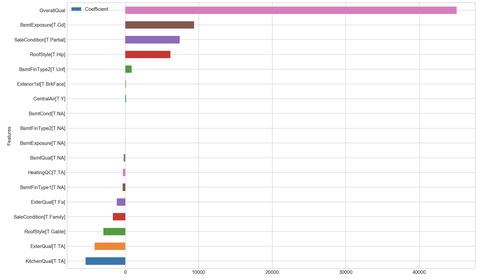
Graph above showed the Top 3 estimators of renovatable features were :
- OverallQual: Rates the overall material and finish of the house
- BsmtExposure: Gd Good Exposure
- SaleCondition: Partial Home was not completed when last assessed (associated with New Homes)
reno_feature_positive_increase_SP['OverallQual'].value_counts()

'''
6.0    30
5.0    18
7.0    17
8.0    12
9.0     4
4.0     3
Name: OverallQual, dtype: int64
'''fig, axes = plt.subplots(nrows=1, ncols=2, figsize=(15,7))
ax0, ax1 = axes.flatten()
sns.distplot(reno_feature_positive_increase_SP['OverallQual'], ax=ax0)
sns.distplot(reno_feature_positive_increase_SP['OverallCond'], ax=ax1)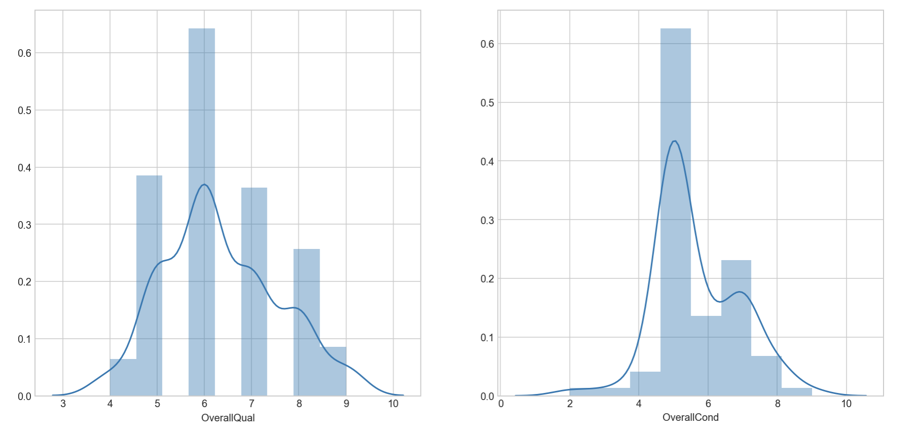
As data at this point already filtered down to only those with positive increase in SalePrice due to renovation, The plot above showed that :
- Overall Qual shall be 6 and above
- Overall Condition shall be 5 and above
A sub-dataframe was formed in order to compare renovatable features vs total no. of units with positive increase in price due to that feature
count_plot_data = reno_feature_positive_increase_SP[renovatable_features].drop(['OverallQual','OverallCond','Id', 'SalePrice'], axis=1)
key = []
count_sum_positive_renoEffect = []
for col in count_plot_data.columns:
key.append(col)
count_sum_positive_renoEffect.append(count_plot_data[col].values.sum())
count_plot_df = pd.DataFrame()
count_plot_df['Feature'] = key
count_plot_df['Total_unit_positive_reno_effect'] = count_sum_positive_renoEffect
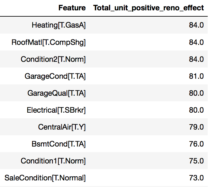
count_plot_df.sort_values(['Total_unit_positive_reno_effect'], ascending=False)Partial view of the tabulated sub-dataframe as below :
effective_reno_features_positive_predictedSP = count_plot_df[count_plot_df['Total_unit_positive_reno_effect']!=0]
effective_reno_features_positive_predictedSP.sort_values('Total_unit_positive_reno_effect', ascending=True).plot(x='Feature', y='Total_unit_positive_reno_effect', kind='barh', figsize=(15,50))
plt.show()
Partial view of the renovatable features as below :
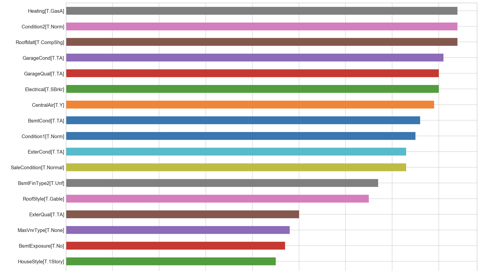
Top 3 estimators of renovatable features were found as :
1) OverallQual: Rates the overall material and finish of the house
- [OverallQual shall be 6 and above ]
- [OverallCondition shall be 5 and above]
2) BsmtExposure: Refers to walkout or garden level walls
- [Good Exposure]
3) SaleCondition: Partial Home was not completed when last assessed (associated with New Homes)
- [Normal Sale]
Others renovatable features to consider :
- Heating : Gas forced warm air furnace
- Condition2 : Normal proximity to various conditions (if more than one is present)
- RoofMatl: Roof material Standard (Composite) Shingle
2.4 Model Robustness :
Should it be used to evaluate which properties to buy and fix up?
Key tables for both Fix features and Mix features were reviewed again to have an overview for commentary purpose
Mean_Prediction_Gap_Mix = np.mean(merge_table_mix_fix['Absolute Prediction Gap in $_Mix'])
Mean_Prediction_Gap_Fix = np.mean(merge_table_mix_fix['Absolute Prediction Gap in $_Fix'])
Mean_Cost_of_reno_effect = np.mean([abs(v) for v in cost_effect_comparison['Cost of Renovation Effect']])

print('Mean_Prediction_Gap_Mix \t:{}'.format(Mean_Prediction_Gap_Mix))
print('Mean_Prediction_Gap_Fix \t:{}\n'.format(Mean_Prediction_Gap_Fix))
print('Absolute value of renovation effect [Mean_Cost_of_reno_effect]')
print(Mean_Cost_of_reno_effect)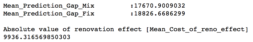
On average, the renovation didn’t really add into higher saleprice justified based on fix features. Fix features were found still the key factors determining the SalePrice
print('Model_used \t\t\t: LassoCV')
print('Score_achived \t\t\t: {}'.format(score_fix))
print('No_of_variables_involved \t: {}'.format(no_of_variables_in_modeling2))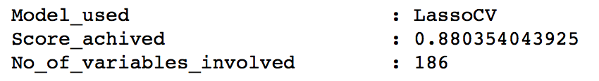
Based on the score, it was considered moderate enough to be used to assist decision making on investment potential. However, there were 186 variables needed in order to achive this score. Data completeness, data quality and data integrity were therefore very important and critical for model performance and accuracy. It was thus advisable to use it as reference and continue monitoring, timely adjustment would still be needed.
Project Summary :
Part 1 : Home Value Prediction based on Fixed Characteristics
'2nd model_all fix features :\nscore = {}\t no_of_feature = {}\t MAE:{}\t MSE:{}\t RMSE: {}'.format(score_fix, no_of_variables_in_modeling2, MAE_2, MSE_2, RMSE_2))
print('Top 2 estimators :\n1. GrLivArea: Above grade (ground) living area square feet; 2. Neighborhood[T.NridgHt]: Northridge Heights')
The model built for home value prediction was using Lasso CV with score of 0.88. It involved 186 feautes with various mean errors as shown above. Top 2 feature estimators were found as Ground Living Area and Neighborhood at Northridge Heights
Part 2 : Validation on value of changeable property characteristics unexplained by the fixed ones.
Top 3 highest coefficients could be used as estimators for higher achievable predicted saleprice as below
- GrLivArea: Above grade (ground) living area square feet
- OverallQual: Rates the overall material and finish of the house
- Neighborhood: Northridge Heights
However, for cost of effects from renovatable features, Tope 3 estimators were found to be:
- OverallQual: Rates the overall material and finish of the house
- in which [OverallQual shall be 6 and above ] and [OverallCondition shall be 5 and above]
- BsmtExposure: Refers to walkout or garden level walls
- in which condition should be rated as Gd ( Good Exposure )
- SaleCondition: Partial Home was not completed when last assessed (associated with New Homes)
- in which condition to be at least as Normal Sale type
Others renovatable features to consider including the followings :
- Heating : To be with Gas forced warm air furnace
- Condition2 : Normal proximity to various conditions (if more than one is present)
- RoofMatl: To have standard ( composite ) Shingle roof material
For return of investment on renovatable features, the difference between fix features vs renovatable features were found as below :
The renovation didn’t really add into higher saleprice justified based on fix features. Fix features were found still the key factors determining the SalePrice
As for overall model performance :
it was considered moderate enough to be used to assist decision making on investment potential. However, there were 186 variables needed in order to achive this score. Data completeness, data quality and data integrity were therefore very important and critical for model performance and accuracy. It was thus advisable to use it as reference and continue monitoring, timely adjustment would still be needed.