
In the domain of analysing company growth and its potential, the conventional way is normally conducted by checking the comprehensive financial reports and operation status. However, to many who do not really hold lots of business insights and sufficient financial figures, is there a simpler but yet statistically studied method that they can use as a baseline reference ?
The objective of the project is to attempt using limited information and small set of features to predict the company potential if the company will eventually go for IPO or acquired by other market players. It is not meant to serve as any financial or investment advice but more a project to exercise and integrate various modelling trials to assist the preliminary assessment decision in a more structure and statistically explainable approach.
The outcomes of the data analysis and model prediction provide moderate information on the competitive landscape across various market sectors while modelling the growth potential of various companies that were in focus by the Top 10 key investors.
Goal
To identify high growth company & predict its potential for successful IPO / acquisition

Success Metrics
- Focusing on True Positive Rate [ Sensitivity ]
- Company predicted as Acquired/IPO does get acquired/IPO in real world
- Target Recall Score for True Positive > 70%
- Dianogstic of Binary Classification Performance
- To assess using Receiver Operating Characteristic curve ( ROC curve ) , a graphical plot that illustrates the diagnostic ability of a binary classifier system as its discrimination threshold is varied
- Target ROC_AUC score > 70%
Data Source
- Raw dataset from Crunchbase @ 2015
- Missing values handling via Web-scrapped data
- Validation via Web-scapped / direct webpage data @ 2018
Analytical Approach
1. Scope Definition to Focus on Market Sectors of High Interest
Since available data set was back to 2015, start up companies to focus for the analysis shall not be funded too many years back.
- Criteria 1: Limit scope to companies with last round of funding obtained at 2010 and beyond
- Criteria 2: Restrict analysis to only funding sources coming from:
- venture capitalist
- seed funding
- angel investor
- private_equity
- Criteria 3: Extraction of data involving investments done by top 10 investors
2. Thorough Data Mining & Cleaning
Data cleansing and filtration based on scopes defined and perform preliminary basic analysis to get the most relevant data out for next level of details analysis
3. Exploratory Data Analysis
- Extraction of Top10 Key Investors based on the Total Investment Amount in USD
- Reclassification of Market Sector and group scatterred sectors into the closest business fields
- Similarity of Investment Porfolio via Network Graph
- Missing Values Handling and Replacement via Web-Scrapping
- Preliminary Statistical Analysis for
- Acquired companies
- IPO companies
- Closed down companies
4. Sampling Methods & Predictive Model Selection
- Evaluation of various sampling methods for Imbalanced datasets
- Evaluation of various classification models for best predictive model selection
5. Data Validation for Predictive Model Improvement
- Validation of False Positive data versus latest state in 2018
- Recalculation with latest state to check the actual predictive model performance
Analytical Outcomes
1. Finalization of Top10 Key Investors
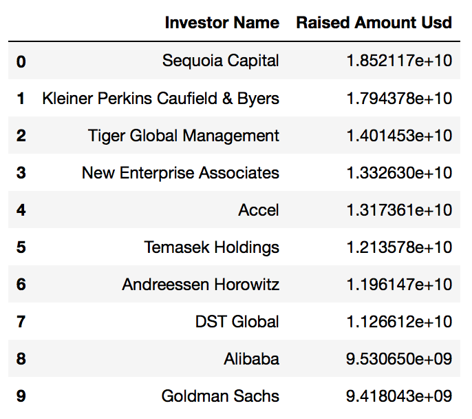
// top 10 investors by amount raised_usd

df_top10_investors.sort_values('Raised Amount Usd', ascending=True).plot(x='Investor Name', y='Raised Amount Usd', kind='barh', figsize=(15,4), colormap='plasma')
plt.title('Total Investment Amount in USD by Top 10 Investors')
plt.show()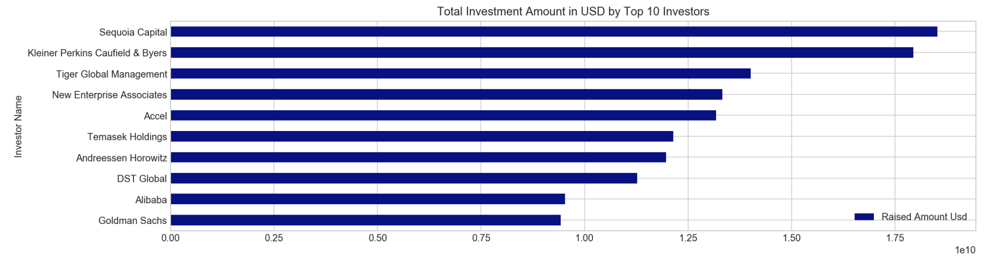
2. Market Sectors In Focus by Top10 Key Investors
// attempt to use TF-IDF vectorizer on company category to check which key words have higher importance/appearance

from sklearn.feature_extraction.text import CountVectorizer, TfidfVectorizer
tvec = TfidfVectorizer(stop_words='english', min_df=1, ngram_range=(1,2), max_features=1000)
// use ngram(1,2) because category is more relevant when mentioning in single (software), or pair words (consumer electronics)

tvec.fit(df_top10investor_choice['company_category_list_2'])
df_catModified_tvec = pd.DataFrame(tvec.transform(df_top10investor_choice['company_category_list_2']).todense(), columns=['Category_'+ v for v in tvec.get_feature_names()], index=df_top10investor_choice['company_category_list_2'].index)

wordcount = df_catModified_tvec.sum().sort_values(ascending=False)
df_wordcount = pd.DataFrame(wordcount)
df_wordcount = df_wordcount.reset_index()
df_wordcount.rename(columns={'index': 'Feature', 0: 'VectorizerCount'}, inplace=True)
df_wordcount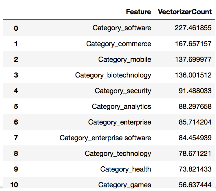
// market sector sorted by amount raised_usd from top 10 investors

df_MarketSector.sort_values('Raised Amount Usd', ascending=True).plot(y='Raised Amount Usd', x='Market_Sector', kind='barh', figsize=(15,10),colormap='tab20c')
plt.title('Total Investment Amount in USD by Market Sector')
plt.show()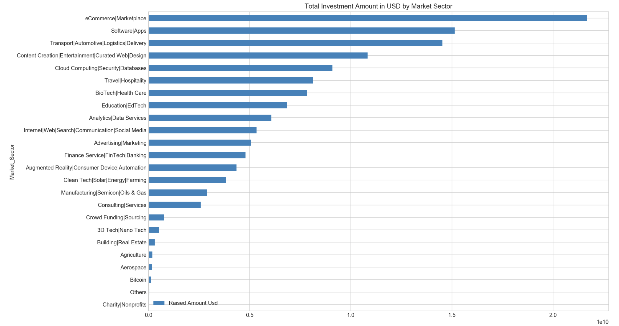
3. Similarity of Investment Portfolio via Network Graph
- 1st Visualization via networkx library
// refine network graph to have visibility on Market Sectors & the common interest among various top 10 investors. An overview that includes investors' path.

import networkx as nx
import matplotlib.pyplot as plt
G = nx.Graph()

// set up nodes
for node in nodes:
    G.add_node(node)

// set up edges
edlabel = []
graph_tuple = []
for i,r in edges_df.iterrows():
    G.add_edge(r['Source'],r['Target'])
    edlabel.append(r['Edge_labels'])
    graph_tuple.append((r['Source'], r['Target']))

// set up edges_labels
edge_labels = dict(zip(graph_tuple, edlabel))

// network graph plot
plt.figure(figsize=(18,12))
pos = nx.shell_layout(G)

nx.draw_networkx_nodes(G,pos)
nx.draw_networkx_edges(G,pos)
nx.draw_networkx_labels(G,pos,labels=nodes_label)
nx.draw_networkx_edge_labels(G,pos, edge_labels=edge_labels)
plt.show()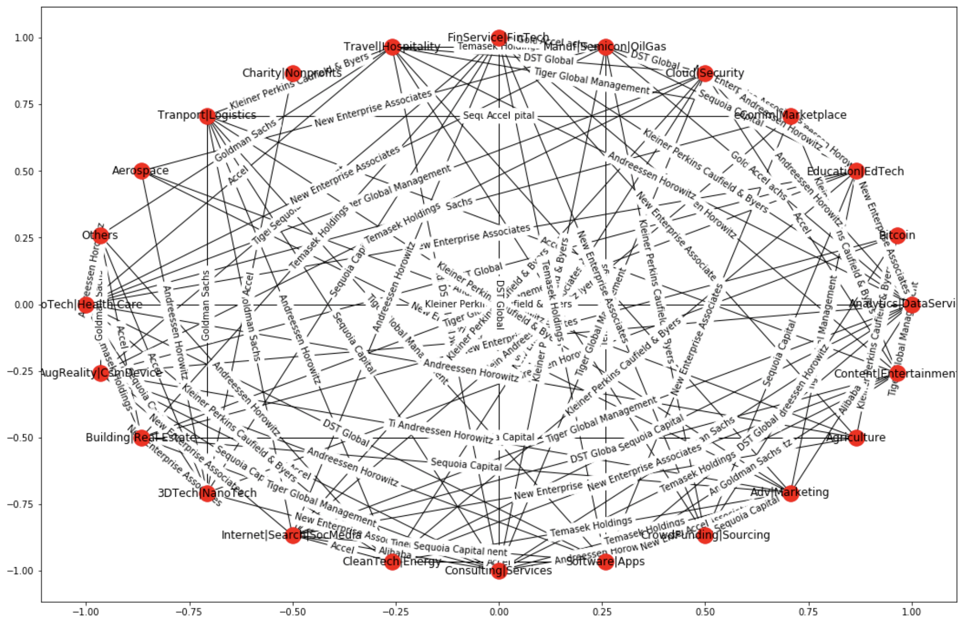
- 2nd Visualization via Neo4j Graph Platform
// codes used in Neo4j for interactive graph plotting

CREATE CONSTRAINT ON (i:Investor) ASSERT i.inv_name IS UNIQUE;
CREATE CONSTRAINT ON (m:MktSector) ASSERT m.sector IS UNIQUE;

LOAD CSV WITH HEADERS FROM "file:///15_df_neo_final.csv" AS line
WITH line
MERGE (i:Investor {inv_name: line.Investor_name})
MERGE (m:MktSector {sector: line.Market_Sector_neo})
CREATE (i)-[:INVESTED_IN]->(m);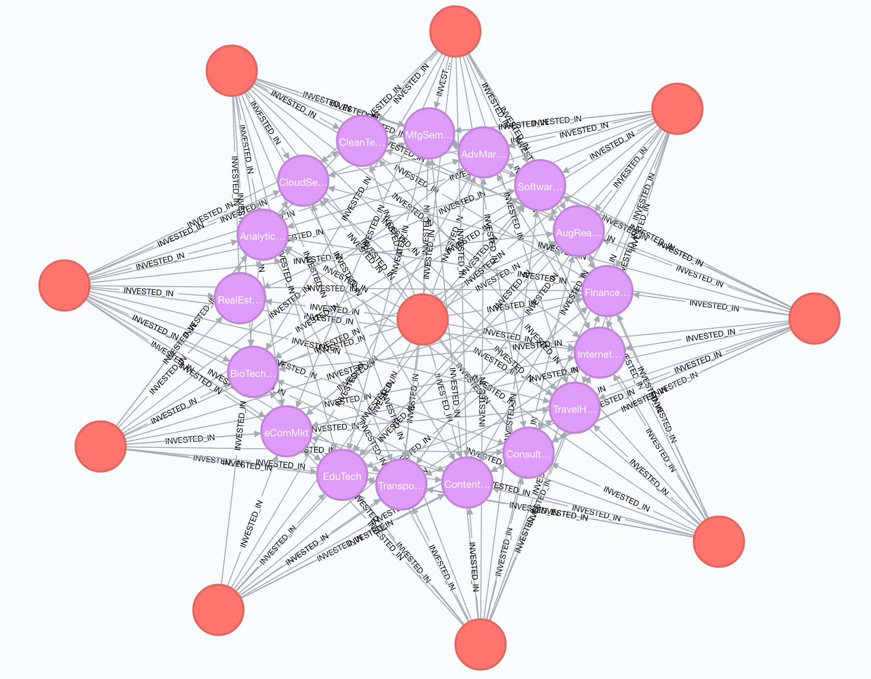
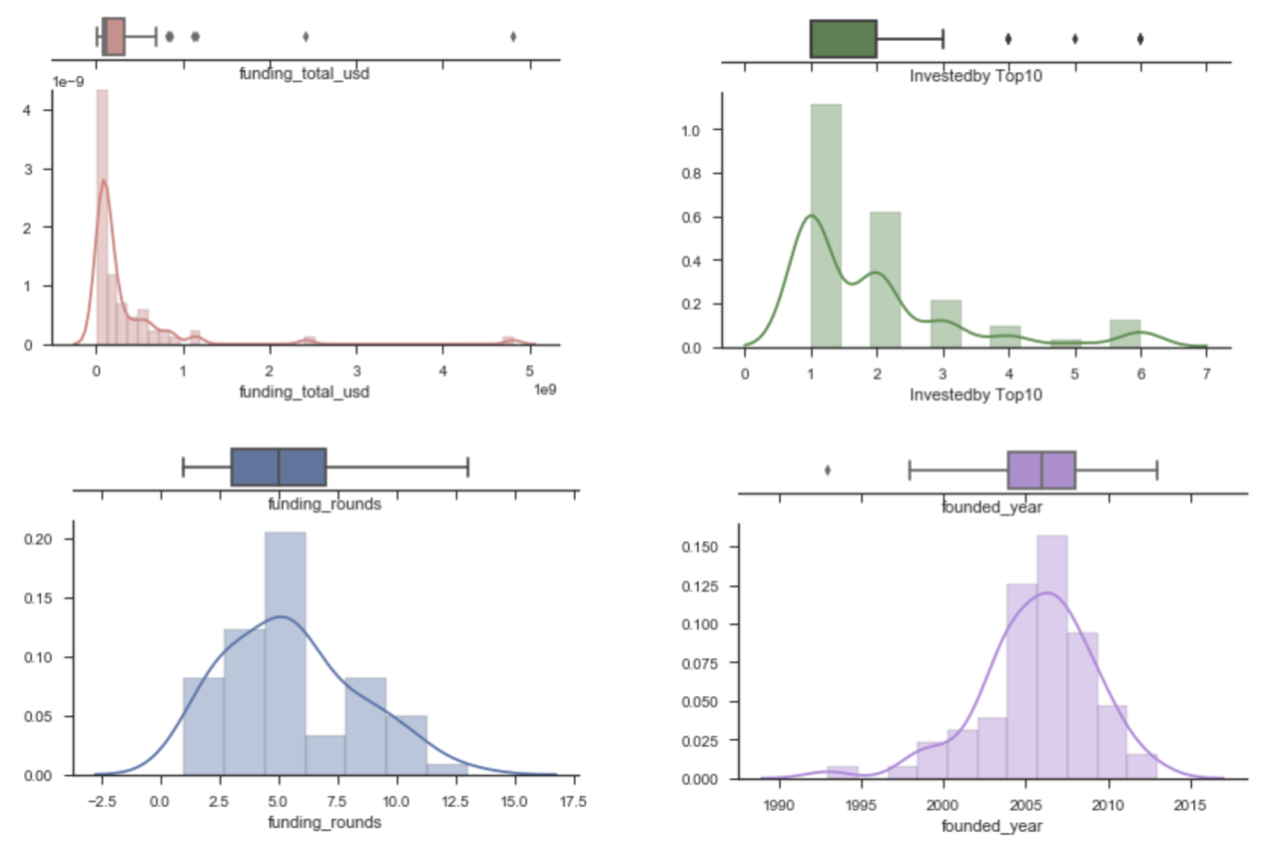
Analysis on Acquired Companies
sns.set(style="ticks")

// Funding Total in USD
x1 = startup_2010onwards[~(startup_2010onwards['funding_total_usd']==0)]['funding_total_usd']
f, (ax_box, ax_hist) = plt.subplots(2, sharex=True,
                                    gridspec_kw={"height_ratios": (.15, .85)})
sns.boxplot(x1, ax=ax_box, color='#e77c7c')
sns.distplot(x1, ax=ax_hist, color='#e77c7c')

ax_box.set(yticks=[])
sns.despine(ax=ax_hist)
sns.despine(ax=ax_box, left=True)

// funding rounds
x2 = startup_2010onwards['funding_rounds']
f, (ax_box, ax_hist) = plt.subplots(2, sharex=True,
                                    gridspec_kw={"height_ratios": (.15, .85)})
sns.boxplot(x2, ax=ax_box)
sns.distplot(x2, ax=ax_hist)

ax_box.set(yticks=[])
sns.despine(ax=ax_hist)
sns.despine(ax=ax_box, left=True)

// No.of Investors from Top10 Investors
x3 = startup_2010onwards['Investedby Top10']
f, (ax_box, ax_hist) = plt.subplots(2, sharex=True,
                                    gridspec_kw={"height_ratios": (.15, .85)})
sns.boxplot(x3, ax=ax_box, color='#388E3C')
sns.distplot(x3, ax=ax_hist, color='#388E3C')

ax_box.set(yticks=[])
sns.despine(ax=ax_hist)
sns.despine(ax=ax_box, left=True)

// years_to_exit
x4 = startup_2010onwards['years_to_exit']
f, (ax_box, ax_hist) = plt.subplots(2, sharex=True,
                                    gridspec_kw={"height_ratios": (.15, .85)})
sns.boxplot(x4, ax=ax_box, color='#bd7ee1')
sns.distplot(x4, ax=ax_hist, color='#bd7ee1')

ax_box.set(yticks=[])
sns.despine(ax=ax_hist)
sns.despine(ax=ax_box, left=True)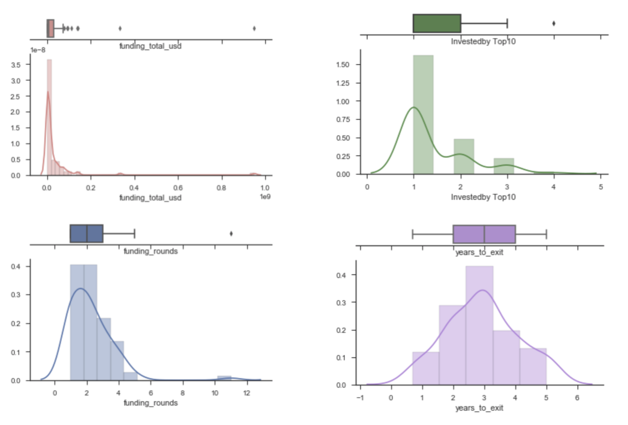
// to check which market sector having the highest chance of being acquired

df_acquired_sortby_MS.sort_values('No_acquired_comp',ascending=True).plot(x='Market_Sector',y='No_acquired_comp', kind='barh', figsize=(15,7), colormap='tab10')
plt.title('No. of Company Exited due to Acquisition')
plt.show()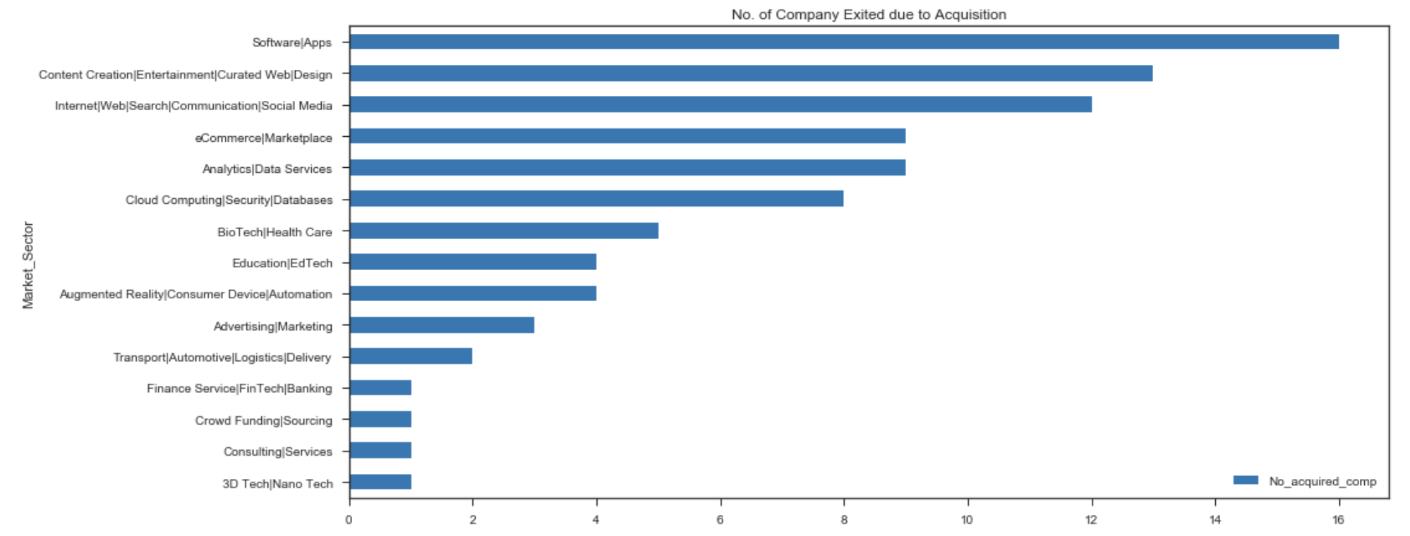
df_acquired_sortby_MS = startup_2010onwards.groupby('Market_Sector')['name'].count().to_frame()
df_acquired_sortby_MS.reset_index(inplace=True)
df_acquired_sortby_MS.rename(columns={'name':'No_acquired_comp'}, inplace=True)
df_acquired_sortby_MS.sort_values('No_acquired_comp', ascending=False, inplace=True)
df_acquired_sortby_MS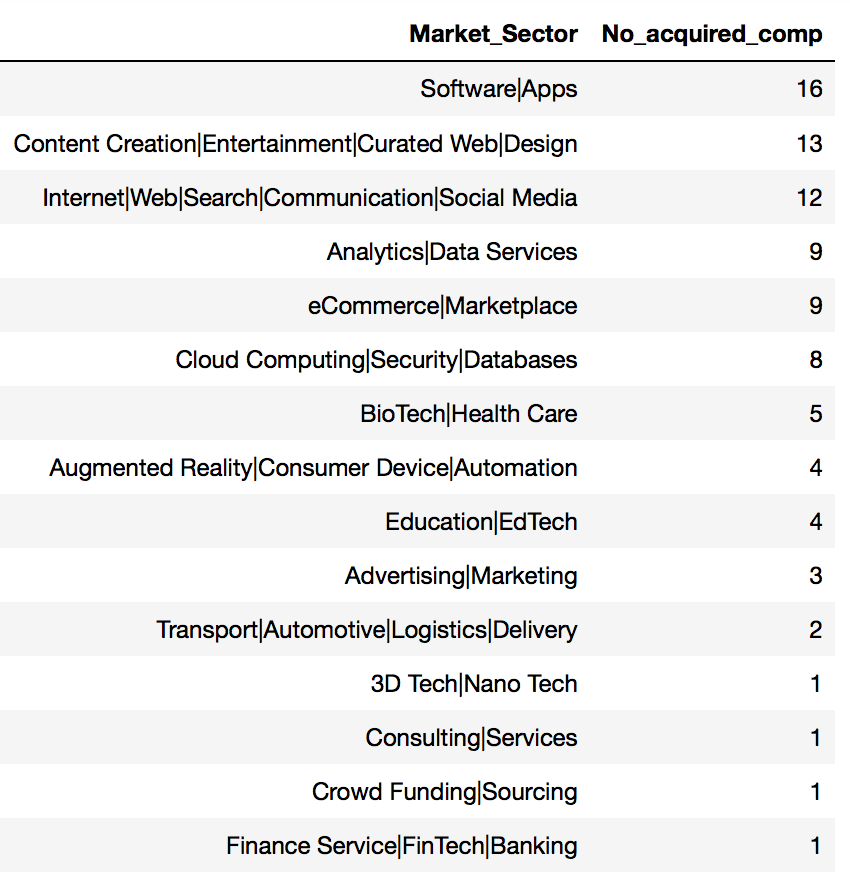
Summary of companies under Top10 investor list that were exited due to acquisition :
- 196 / 1675 companies from top 10 investors list was acquired
- 11.70% acquisition successful rate
For companies founded since 1994
| Average | Median |
|---|---|
| 5.63 years to exit | 5 years |
| 3.09 funding_rounds | 3 |
| 1.56 investor from Top10 investors | 1 |
| $66.67M total funding | $30M |
For start-ups founded 2010 onwards [88 companies]
| Average | Median |
|---|---|
| 2.95 years to exit | 3 years |
| 2.25 funding_rounds | 2 |
| 1.42 investor from Top10 investors | 1 |
| $35.79M total funding | $8.25M |
Top 3 market sectors with higher no. of companies being acquired
- Software\Apps
- Content Creation\Entertainment\Curated Web\Design
- Internet\Web\Search\Communication\Social Media
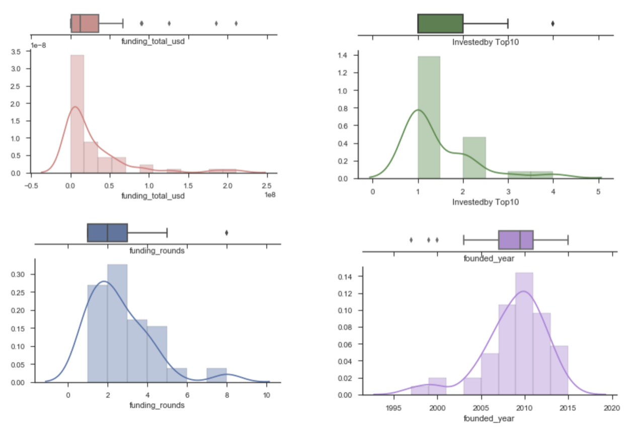
Analysis on IPO Companies
Similar stats analysis approach as done for Acquired companies was repeated and used to study IPO companies. Below are the graphical analytic outcomes for IPO companies :
// to check which market sector having the highest chance of going for IPO

df_ipo_sortby_MS.sort_values('No._IPO_Company',ascending=True).plot(x='Market_Sector',y='No._IPO_Company', kind='barh', figsize=(15,6), colormap='tab10')
plt.title('No. of IPO Companies by Market Sector')
plt.show()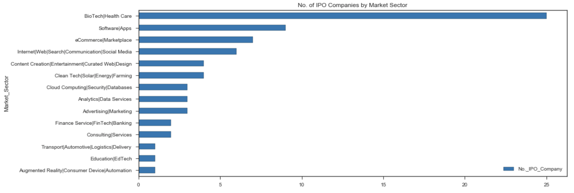
df_ipo_sortby_MS = df_ipo.groupby('Market_Sector')['Company Name'].count().to_frame()
df_ipo_sortby_MS.reset_index(inplace=True)
df_ipo_sortby_MS.rename(columns={'Company Name':'No._IPO_Company'}, inplace=True)
df_ipo_sortby_MS.sort_values('No._IPO_Company', ascending=False, inplace=True)
df_ipo_sortby_MS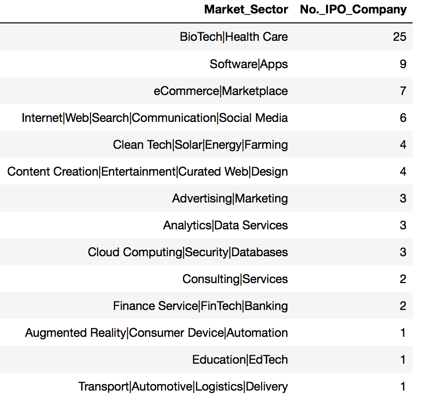
// to check which IPO companies having the highest funding_total

df_ipo_sortby_MS.sort_values('Funding_Total_Usd',ascending=True).plot(x='Company Name',y='Funding_Total_Usd', kind='barh', figsize=(15,30), colormap='tab10')
plt.title('Funding Total in USD by IPO Company')
plt.show()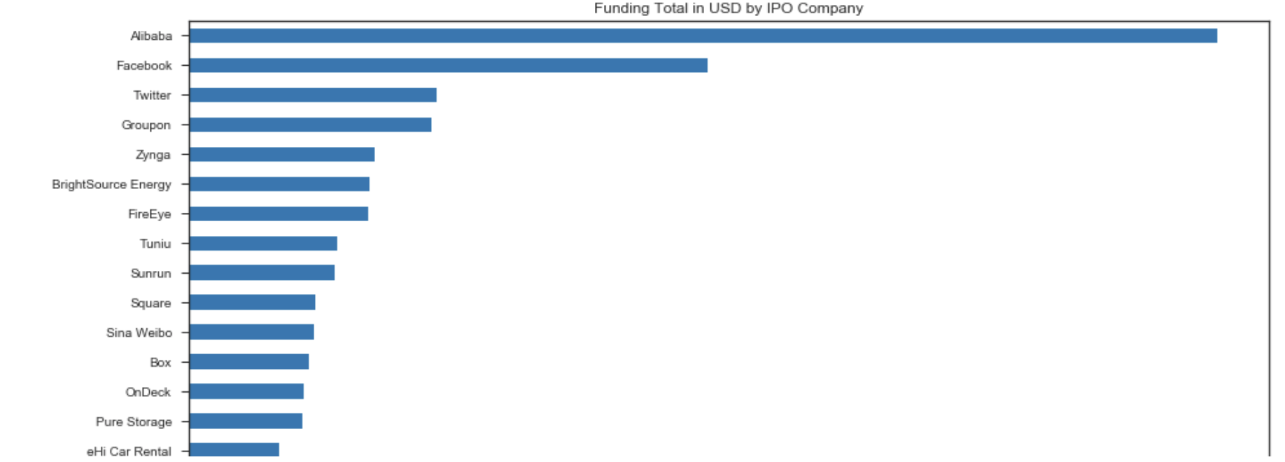
Summary of companies under Top10 investor list that were IPO successfully :
- 71 / 1674 companies were successfully listed
- 4.24% successful IPO rate
From 71 IPO companies :
| Average | Median |
|---|---|
| $332.91M total funding | $112.79M |
| 5.51 funding_rounds | 5 |
| 1.94 investor from Top10 investors | 1 |
| 2005 years to exit | 2006 |
Top 3 Market Sectors having the highest no. of IPO companies:
- BioTech\Health Care : 25
- Software\Apps : 9
- eCommerce\Marketplace : 7
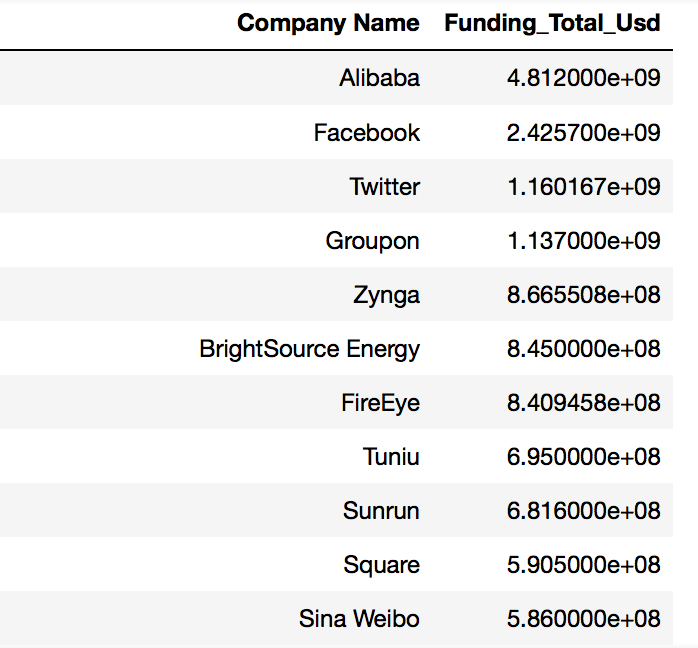
Top 3 IPO companies having the highest funding total:
| Company | Total_Funding |
|---|---|
| 1st Alibaba | $4.81 Billion |
| 2nd Facebook | $2.43 Billion |
| 3rd Twitter | $1.16 Billion |
Analysis on Closed Down Companies
Similar stats analysis approach was again repeated and used to study Closed Down companies. Below are the graphical analytic outcomes for Closed Down companies :
// to check which market sector having the highest no. of closed companies

df_closed_sortby_MS.sort_values('No._closed_Company',ascending=True).plot(x='Market_Sector',y='No._closed_Company', kind='barh', figsize=(15,6), colormap='tab10')
plt.title('No. of Closed Down Companies by Market Sector')
plt.show()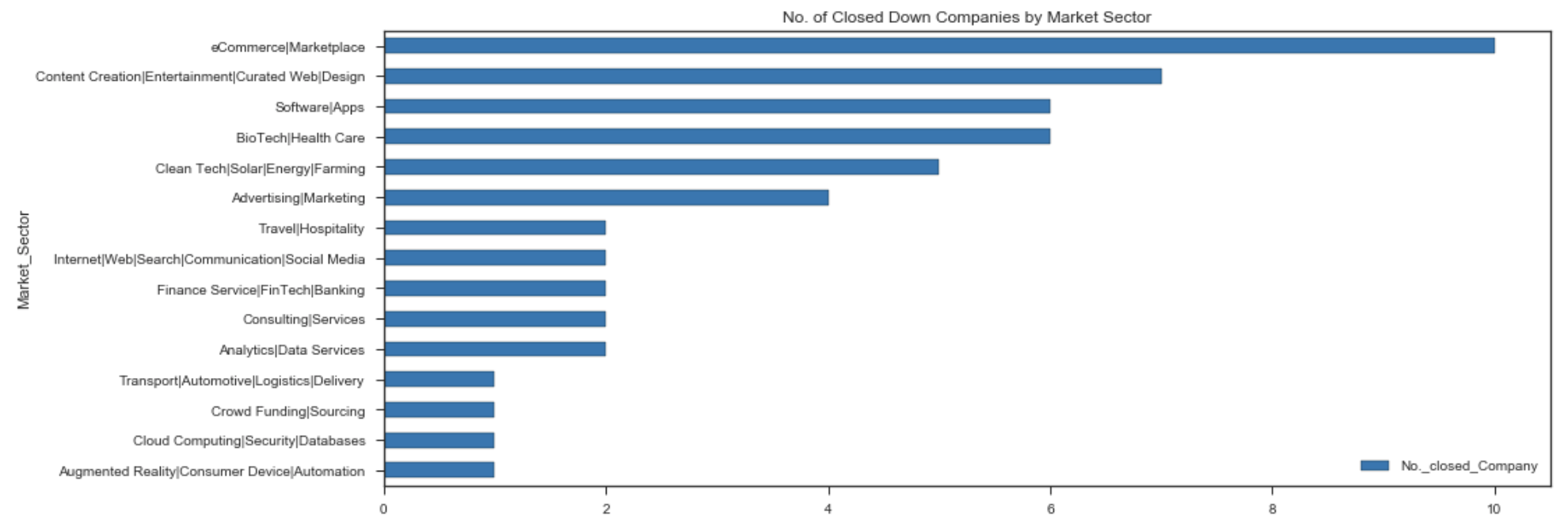
df_closed_sortby_MS = df_closed.groupby('Market_Sector')['Company Name'].count().to_frame()
df_closed_sortby_MS.reset_index(inplace=True)
df_closed_sortby_MS.rename(columns={'Company Name':'No._closed_Company'}, inplace=True)
df_closed_sortby_MS.sort_values('No._closed_Company', ascending=False, inplace=True)
df_closed_sortby_MS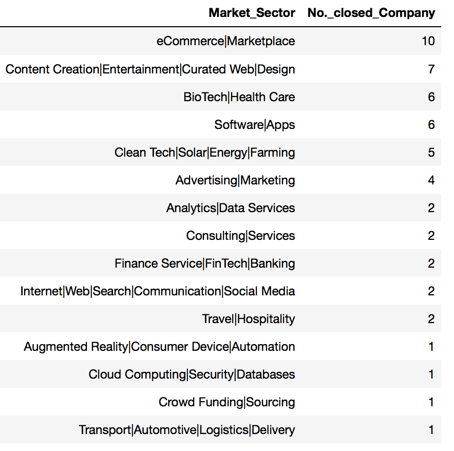
Summary of companies under Top10 investor list that were closed down :
- 52 / 1674 companies were closed down
- 3.11% failure rate
From 52 closed down companies :
| Average | Median |
|---|---|
| $28.66M total funding | $12.15M |
| 2.56 funding_rounds | 2 |
| 1.42 investor from Top10 investors | 1 |
| 2008 years to exit | 2009 |
[ 2008 Subprime Mortgage Financial Crisis ]
Top 3 Market Sectors having the highest no. of Closed Down companies:
- eCommerce\Marketplace : 10
- Content Creation\Entertainment\Curated Web\Design : 7
- BioTech\Health Care : 6
- Software\Apps : 6
Sampling Methods & Predictive Model Selection
Current data set was found not suitable for a comprehensive Time Series Analysis due to the lack of important key feature of Date/Time and its completeness to support continuous time-dependent analysis. With this, pior to starting next core modelling, a new dataframe was set up to exclude companies with Closed Down status and companies that were either acquired or IPO were then combined as one category. The restructure of such dataframe was done in preparation for classification modelling purpose.
- Restructure 1: Exclude companies with Closed Down status
- Restructure 2: Combine acquired companies and IPO companies as one new category
1. Dataframe Readiness
// Create X matrix

X = pd.concat([df_model_2clusters.drop(['Company Name','Market_Sector','Is_Acquired_IPO'], axis=1),mkt_sec], axis=1)
print(X.shape)
X
// create y
y = df_model_2clusters['Is_Acquired_IPO']
y.value_counts()
'''
0 1337
1 266
Name: Is_Acquired_IPO, dtype: int64
'''
// imbalance dataset observed2. Model Preprocessing
// train test split
from sklearn.model_selection import train_test_split

X_train, X_test, y_train, y_test = train_test_split(X, y, test_size=0.3, random_state=42)
from sklearn.preprocessing import StandardScaler
ss = StandardScaler()
Xs_train = ss.fit_transform(X_train)
Xs_test = ss.fit_transform(X_test)3. Sampling Method Evaluation
Since imbalanced dataset was observed, additional step was therefore needed to evaluate sampling methods to balance them before modelling. Logistic RegressionCV was chosen as base model to support this sampling method evaluation since it was the simplest classification model.
Sampling Methods to evaluate as listed below :
- Over Sampling_RandomOverSampler
- Over Sampling_SMOTE
- Combine Sampling_SMOTEENN
- Combine Sampling_SMOTETomek
- Under Sampling_RandomUnderSampler
- Under Sampling_CondensedNearestNeighbour
// Standard Scaler + Random over sample minority class
from imblearn.over_sampling import RandomOverSampler

ros = RandomOverSampler(ratio='minority', random_state=42)
X_ros_train, y_ros_train = ros.fit_sample(Xs_train, y_train)
print('X shape: {}, y shape: {}'.format(X_ros_train.shape, y_ros_train.shape))

'''
X shape: (1874, 27), y shape: (1874,)
'''
// A function used to plot confusion matrix for all evaluated models
def plot_confusion_matrix(cm, classes,
normalize=False,
title='Confusion matrix',
cmap=plt.cm.Blues):
"""
This function prints and plots the confusion matrix.
Normalization can be applied by setting `normalize=True`.
"""
if normalize:
cm = cm.astype('float') / cm.sum(axis=1)[:, np.newaxis]
print('Confusion matrix, after normalization')
else:
print('Confusion matrix, without normalization')
print(cm)
plt.imshow(cm, interpolation='nearest', cmap=cmap)
plt.title(title)
plt.colorbar()
tick_marks = np.arange(len(classes))
plt.xticks(tick_marks, classes, rotation=45)
plt.yticks(tick_marks, classes)
fmt = '.2f' if normalize else 'd'
thresh = cm.max() / 2.
for i, j in itertools.product(range(cm.shape[0]), range(cm.shape[1])):
plt.text(j, i, format(cm[i, j], fmt),
horizontalalignment="center",
color="white" if cm[i, j] > thresh else "black")
plt.tight_layout()
plt.ylabel('True label')
plt.xlabel('Predicted label')'''
--------------------------------------------------------------
Base model for Sampling Method Trial : Logistic RegressionCV
--------------------------------------------------------------
'''
from sklearn.linear_model import LogisticRegressionCV
from sklearn.metrics import confusion_matrix, classification_report
print('------------------------------------------------------------------')
print('Performance Check for Model : LogisticRegressionCV_SS+RoS')
print('with Preprocessing Method : Over Sampling - RandomOverSampler')
print('------------------------------------------------------------------')
print('\n')
// with random over sampler + std scaler
s1_model_LOGR1 = LogisticRegressionCV(cv=5)
s1_model_LOGR1.fit(X_ros_train, y_ros_train)
s1_y_predictions_LOGR1 = s1_model_LOGR1.predict(Xs_test)
s1_y_prob_predictions_LOGR1 = s1_model_LOGR1.predict_proba(Xs_test)
print('score_LogisticRegressionCV_SS+ROS \t= {}'.format(round(s1_model_LOGR1.score(Xs_test, y_test),4)))
print('\n')
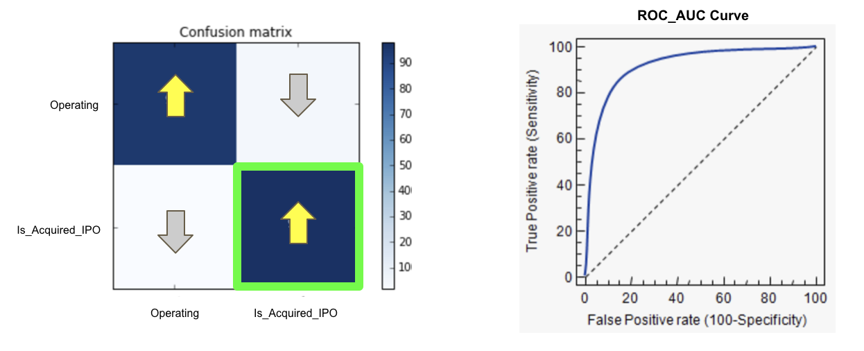
// Compute confusion matrix
cnf_matrix = confusion_matrix(y_test, s1_y_predictions_LOGR1)
np.set_printoptions(precision=2)
class_names = ['Operating','Acquired/IPO']
// Plot non-normalized confusion matrix
plt.figure()
plot_confusion_matrix(cnf_matrix, classes=class_names,
title='Confusion matrix, without normalization')
plt.show()
// Plot normalized confusion matrix
plt.figure()
plot_confusion_matrix(cnf_matrix, classes=class_names, normalize=True,
title='Confusion matrix, after normalization')
plt.show()
print('Classification report :')
print('------------------------')
print(classification_report(y_test, s1_y_predictions_LOGR1))
print('\n')
s1_roc_auc_score = round(roc_auc_score(y_test, s1_y_prob_predictions_LOGR1[:,1]),4)
print('ROC_AUC score :')
print('----------------')
print(s1_roc_auc_score)
// Plot roc_auc graph to show area under the curve
fpr, tpr, _ = roc_curve(y_test, s1_y_prob_predictions_LOGR1[:,1])
roc_auc = auc(fpr, tpr)
plt.figure(figsize=[6,6])
plt.plot(fpr, tpr, label='ROC curve (area = %0.2f)' % roc_auc, linewidth=4)
plt.plot([0, 1], [0, 1], 'k--', linewidth=4)
plt.xlim([-0.05, 1.0])
plt.ylim([-0.05, 1.05])
plt.xlabel('False Positive Rate', fontsize=12)
plt.ylabel('True Positive Rate', fontsize=12)
plt.title('Companies from Top10 Investor List : Is_Acquired_or_IPO', fontsize=12)
plt.legend(loc="lower right")
plt.show()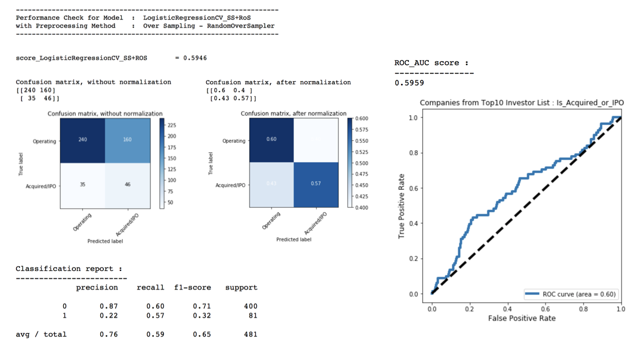
Summary of Sampling Method Evaluation
Set up a summary to tabulate ROC_AUC score and the recall score for Class 1 for the various evaluated sampling methods for easy reference to decide which one to choose for further comprehesive modeling selection
df_summary_SampMethod = pd.DataFrame(columns=['Sampling Method','ROC_AUC score','Recall_score_Class1'])samplingMethod = ['Over Sampling_RandomOverSampler','Over Sampling_SMOTE','Combine Sampling_SMOTEENN','Combine Sampling_SMOTETomek','Under Sampling_RandomUnderSampler','Under Sampling_CondensedNearestNeighbour']rocScore_SampM = [s1_roc_auc_score, s2_roc_auc_score,s3_roc_auc_score,s4_roc_auc_score,s5_roc_auc_score,s6_roc_auc_score]
recallScore_SampM = [round(recall_score(y_test, s1_y_predictions_LOGR1),4), round(recall_score(y_test, s2_y_predictions_LOGR1),4), round(recall_score(y_test, s3_y_predictions_LOGR1),4), round(recall_score(y_test, s4_y_predictions_LOGR1),4), round(recall_score(y_test, s5_y_predictions_LOGR1),4), round(recall_score(y_test, s6_y_predictions_LOGR1),4)]df_summary_SampMethod['Sampling Method'] = samplingMethod
df_summary_SampMethod['ROC_AUC score'] = rocScore_SampM
df_summary_SampMethod['Recall_score_Class1'] = recallScore_SampM
df_summary_SampMethod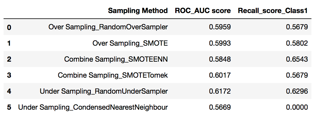
With base model of LogisticRegression CV, scoring for various sampling methods were compared. From the summary table, Under Sampling_Random Under Sampler was observed having the highest ROC_AUC score with recall_score for Class1 was also relatively higher compared to other sampling methods.
Therefore, final sampling method to use for next model selection process is < Under Sampling_Random Under Sampler >
4. Predictive Model Selection
With sampling method finalized above as Random Under Sampler, the data will be preprocessed using Standard scalar followed by this under sampling method in order to achive balanced dataset for subsequent modelling
Classification models to evaluate as listed below :
- Logistic Regression CV
- KNeighbors Classifier
- SGD Classifier
- Gradient Boosting Classifier
- Support Vector Classifier
- Random Forest Classifier
from imblearn.under_sampling import RandomUnderSampler

rds = RandomUnderSampler(ratio='majority', random_state=42)
X_rds_train, y_rds_train = rds.fit_sample(Xs_train, y_train)
print('X shape: {}, y shape: {}'.format(X_rds_train.shape, y_rds_train.shape))

'''
X shape: (370, 27), y shape: (370,)
'''
// -------------------------------------
// 6th trial : Random Forest Classifier
// -------------------------------------
import itertools
from sklearn.ensemble import RandomForestClassifier
from sklearn.metrics import confusion_matrix, classification_report, roc_curve, auc, roc_auc_score
// with random over sampler + std scaler
model_RFC1 = RandomForestClassifier(random_state=42)
model_RFC1_params = {'n_estimators':np.arange(45,55,1),
'criterion':['gini','entropy'],
'max_features':['log2','auto'],
'max_depth':[3,4,5,6]}
RFC1_GS = GridSearchCV(model_RFC1, model_RFC1_params, n_jobs=3, cv=5, verbose=1)
RFC1_GS.fit(X_rds_train, y_rds_train)
y_predict_RFC1_GS = RFC1_GS.predict(Xs_test)
y_prob_predict_RFC1_GS = RFC1_GS.predict_proba(Xs_test)
print(RFC1_GS.best_params_)
print('\n')
print('---------------------------------------------------------------')
print('Performance Check for Model : Random Forest Classifier_SS+RoS')
print('---------------------------------------------------------------')
print('\n')
// Compute confusion matrix
cnf_matrix = confusion_matrix(y_test, y_predict_RFC1_GS)
np.set_printoptions(precision=2)
class_names = ['Operating','Acquired/IPO']
// Plot non-normalized confusion matrix
plt.figure()
plot_confusion_matrix(cnf_matrix, classes=class_names,
title='Confusion matrix, without normalization')
plt.show()
// Plot normalized confusion matrix
plt.figure()
plot_confusion_matrix(cnf_matrix, classes=class_names, normalize=True,
title='Confusion matrix, after normalization')
plt.show()
print('-----------------------------------------------------------------------------------------------------------')
print('Classification report :')
print('------------------------')
print(classification_report(y_test, y_predict_RFC1_GS))
print('-----------------------------------------------------------------------------------------------------------')
print('ROC_AUC score :')
print('----------------')
print(round(roc_auc_score(y_test, y_prob_predict_RFC1_GS[:,1]),4))
// To plot roc_auc graph to show area under the curve
fpr, tpr, _ = roc_curve(y_test, y_prob_predict_RFC1_GS[:,1])
roc_auc = auc(fpr, tpr)
plt.figure(figsize=[6,6])
plt.plot(fpr, tpr, label='ROC curve (area = %0.2f)' % roc_auc, linewidth=4)
plt.plot([0, 1], [0, 1], 'k--', linewidth=4)
plt.xlim([-0.05, 1.0])
plt.ylim([-0.05, 1.05])
plt.xlabel('False Positive Rate', fontsize=12)
plt.ylabel('True Positive Rate', fontsize=12)
plt.title('Companies from Top10 Investor List : Is_Acquired_or_IPO', fontsize=12)
plt.legend(loc="lower right")
plt.show()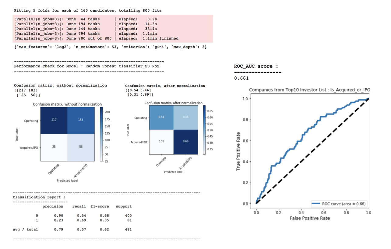
Summary of Predictive Model Selection
Tabulate summary of model performance for ease of model finalization and conclusion wrap up
df_summary_model = pd.DataFrame(columns=['Model','ROC_AUC score','Recall score_Class 1'])

model = ['Logistic Regression CV', 'KNeighbors Classifier','SGD Classifier','Gradient Boosting Classifier',
         'Support Vector Classifier', 'Random Forest Classifier']

rocScore_ModSel = [round(roc_auc_score(y_test, y_prob_predict_LOGR1_GR[:,1]),4), round(roc_auc_score(y_test, y_prob_predict_KNC1_GS[:,1]),4), round(roc_auc_score(y_test, y_prob_predict_SGD1_GS[:,1]),4), round(roc_auc_score(y_test, y_prob_predict_GBC1_GS[:,1]),4), round(roc_auc_score(y_test, y_prob_predict_SVC1_GS[:,1]),4),round(roc_auc_score(y_test, y_prob_predict_RFC1_GS[:,1]),4)]

recallScore_ModSel = [round(recall_score(y_test, y_predict_LOGR1_GS),4), round(recall_score(y_test, y_predict_KNC1_GS),4), round(recall_score(y_test, y_predict_SGD1_GS),4), round(recall_score(y_test, y_predict_GBC1_GS),4), round(recall_score(y_test, y_predict_SVC1_GS),4), round(recall_score(y_test, y_predict_RFC1_GS),4)]


df_summary_model['Model'] = model
df_summary_model['ROC_AUC score'] = rocScore_ModSel
df_summary_model['Recall score_Class 1'] = recallScore_ModSel
df_summary_model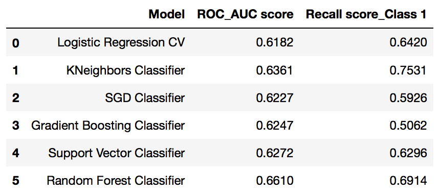
With Grid Search on various models and various parameter trials, the best ROC_AUC score is in the range of 0.60-0.67. Random Forest Classifier was found having the highest ROC_AUC score at 0.66 with Recall score for Class 1 stood 2nd highest at 0.69
Predictive Model Best Estimator & Features Importance
Based on earlier model evaluation on Random Forest Classifier, the best estimators & their parameters as below:
- bootstrap=True
- class_weight=None
- criterion=’gini’
- max_depth=3
- max_features=’log2’
- max_leaf_nodes=None
- min_impurity_decrease=0.0
- min_impurity_split=None
- min_samples_leaf=1
- min_samples_split=2
- min_weight_fraction_leaf=0.0
- n_estimators=53
- n_jobs=1
- oob_score=False
- random_state=42
- verbose=0
- warm_start=False
// Form new dataframe to list down the features and their importance values

df_RFC_features = pd.DataFrame(dict_RFC_features.items(), columns=['Features','Feature_Importance'])
df_RFC_features.sort_values(['Feature_Importance'], ascending=False, inplace=True)

df_RFC_features[df_RFC_features['Feature_Importance']>0]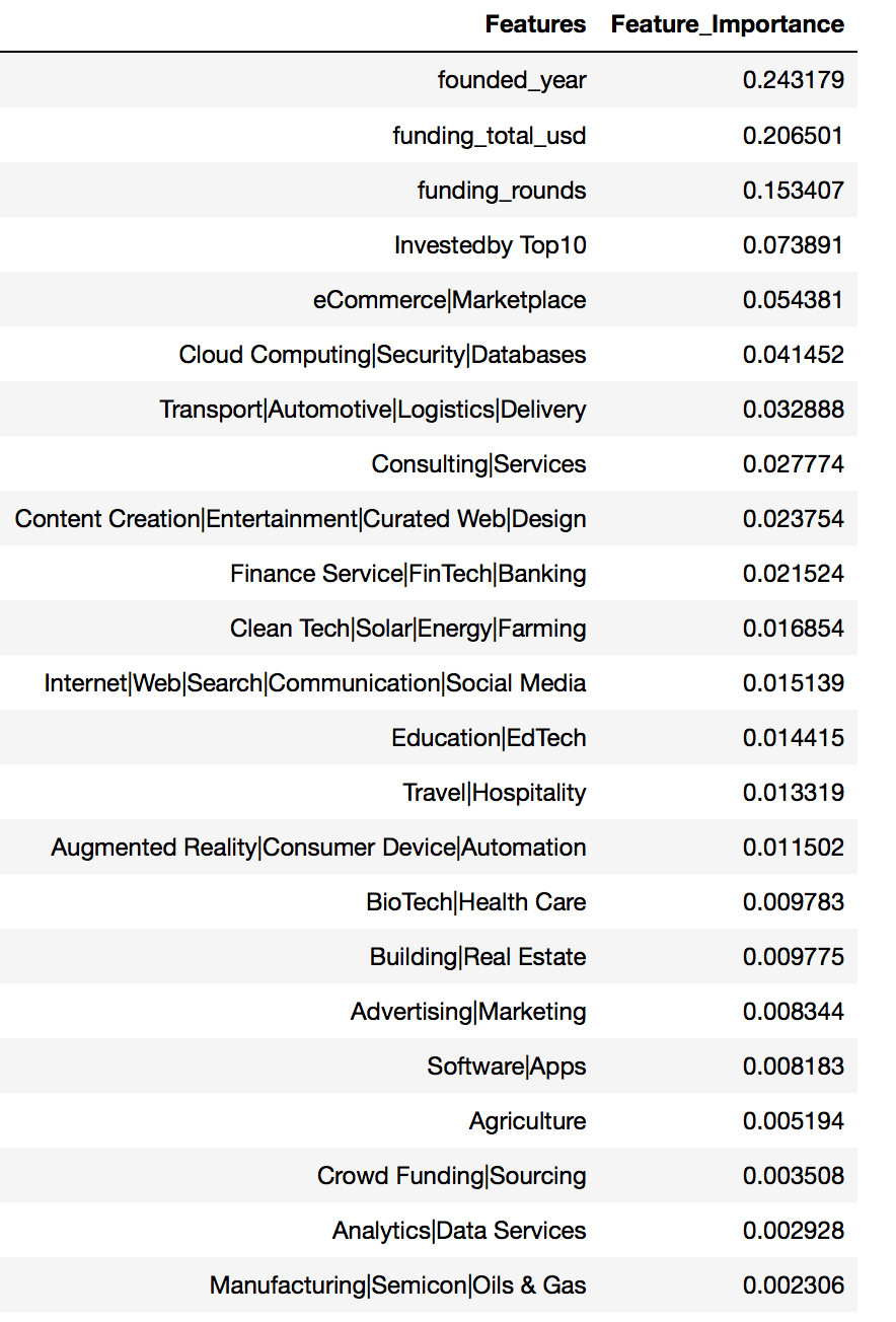
Validation of False Positive with Data @ 2018
Since precision and recall score for Class 1 in Confusion Matrix is not upto expectation, validation of the all False Positive to be done next to check if any of those predicted IPO/acquired companies did get listed/acquired after year 2015
Companies latest status could be validated through web-scrapped script / directly reference on webpage
df_validation['corrected_FalsePositive'] = np.where(df_validation['Validation_2018_rev']=='-',1,0)
df_validation['Validation_2018_rev'].value_counts()

'''
-           146
Acquired     22
IPO          10
Closed        5
Name: Validation_2018_rev, dtype: int64
'''
extra_percent_Acquired_IPO = round(32.0/(146+22+10+5)*100,2)
extra_percent_Acquired_IPO
'''
17.49
'''risk_percent_ClosedDown = round(5.0/(146+22+10+5)*100,2)
risk_percent_ClosedDown
'''
2.73
'''// check updated confusion matrix in dataframe to ensure it is correctly positioned before proceeding to plots
conmat = np.array(confusion_matrix(df_tempVal2['adjusted_Is_Acquired_IPO'], df_tempVal2['y_predict_RFC'], labels=[0,1]))
confusion = pd.DataFrame(conmat, index=['isNot_acquired_IPO', 'is_acquired_IPO'],
columns=['predictedNot_acquired_IPO','predicted_acquired_IPO'])
confusion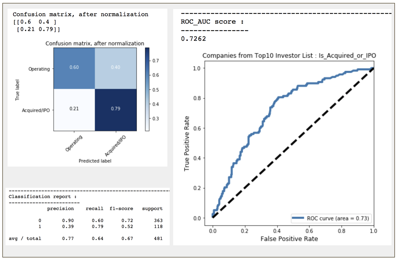
17.49% of companies under false positive were actually acquired/IPO after 2015. Overall recall score for class 1 after factored in the latest company status now inceased from 0.69 to 0.79 ~~
Project Summary
Based on the dataset of 2015, the performance of companies under Top10 Investor List as follows :
196 / 1674 companies from top 10 investors list were acquired
- [ 11.70% acquisition successful rate ]
71 / 1674 companies were successfully listed
- [ 4.24% successful IPO rate ]
52 / 1674 companies were closed down
- [ 3.11% failure rate ]
Due to imbalance dataset, sampling method was therefore applied. Based on highest ROC_AUC score and Recall Score for True Positive, the final selected classification predictive model was Random Forest Classifier coupled with Random Under Sampler Method. The analysis and prediction done based on 2015 data set would yield a Recall score of only 0.69 for True Positive and AUC score of 0.66. Regardless of various hyperparameters tuning and evaluation of different predictive models, the target metrics were still ranging between 0.6 to < 0.7, hitting the limitation of the evaluated features to yield better prediction score.
Subsequent validation of the False Positive data with the latest state as of 2018 showed that there was an additional 32 companies ( ~17.5% of the False Positive ) were acquired/listed after 2015. However, there was also 5 companies ( 2.7% ) were found closed down. As original dataset cut off timeframe was back to 2015, giving longer observation/holding period of 3 years on those predicted high potential/high growth companies, the chances of them getting acquired/listed was around 17% more.
The validation of False Positive with latest company state showed an increase of True Positive Recall score to 0.79 and an adjusted ROC_AUC score was at 0.72. Target of >70% would be achievable only with longer period in this project based on the evaluated predictive model.
With only 5 key features :
- funding_total
- funding_rounds
- no.of key investers
- founding year
- market sectors
in addition to various scatterred data sets, the performance of the model was therefore at moderate level to serve as preliminary baseline to assess a company mid-long term growth potential.